Category: Uncategorized

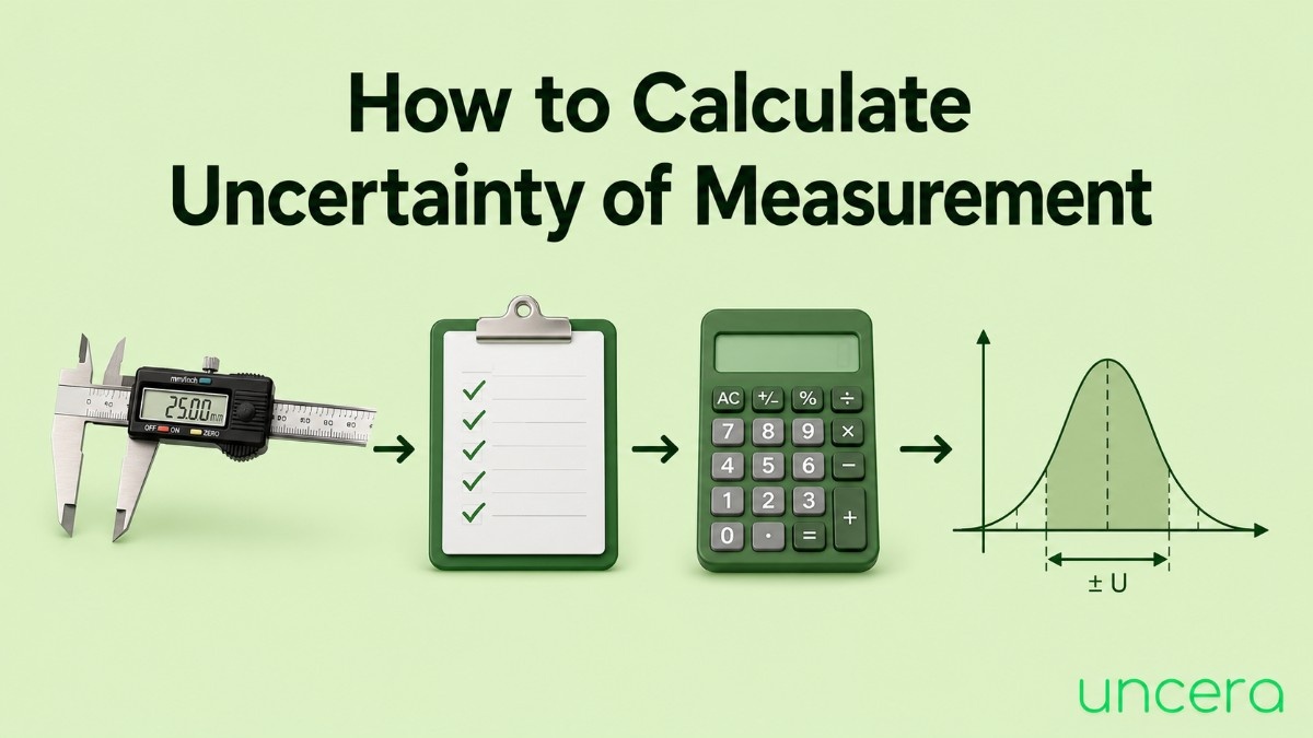
Most people meet measurement uncertainty as a formula on a slide and never quite recover. It looks like statistics homework. It isn’t. It’s bookkeeping you list everything that could make your measurement wrong, put a number on each one, and add them up in a slightly unusual way.

That’s it. Eight steps, and you can do the whole thing in a spreadsheet.

This guide walks through the complete calculation, from your first repeated reading to the ± figure you write on the report. There’s a full worked example partway down, so if you learn better by seeing the numbers move, skip ahead to it and come back.

---

The Short Version

Here’s the whole process in six lines, so you know where this is going:

1. List every source of uncertainty in your measurement.
2. Work out a value for each one.
3. Convert them all into standard uncertainties (the same statistical units).
4. Combine them by squaring, adding, and taking the square root.
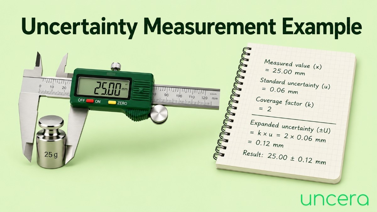
5. Multiply by a coverage factor, usually 2.
6. Report your result as value ± uncertainty.

The two formulas that matter:

Combined standard uncertainty: u꜀ = √(u₁² + u₂² + u₃² + …)

Expanded uncertainty: U = k × u꜀

Everything below is just detail on how to fill in those u values.

---

Before You Calculate Anything: Define the Measurand

This step gets skipped constantly and it causes more trouble than any formula.

The measurand is the specific quantity you’re measuring. Not “the shaft” the diameter of the shaft, at the midpoint of the journal, at 20 °C, measured with an outside micrometer.

Why the fuss? Because your list of uncertainty sources depends entirely on this definition. If your measurand includes “at 20 °C” but you measured at 26 °C, thermal expansion becomes a source you have to account for. If your measurand is “the diameter at the midpoint” but the shaft is slightly tapered, where exactly you placed the micrometer becomes a source too.

Write one clear sentence describing what you’re measuring, under what conditions, with what. Then start listing.

---

Source of Uncertainty

Sit down and brainstorm everything that could shift your reading. Six families cover almost all of them:

• The instrument – resolution, its own calibration uncertainty, drift, wear, hysteresis
• The reference standard – your slip gauge or setting ring has an uncertainty from its own calibration, and it passes straight through to you
• The environment – temperature above all, then vibration, humidity, air pressure
• The operator – measuring force, parallax, alignment, judgement
• The workpiece – roundness, flatness, surface roughness, taper
• The method – clamping, fixturing, probe strategy, how many points and where.

You won’t quantify all of them. Some will turn out to be negligible and you’ll drop them. But list them first and prune later the source you never wrote down is the one that quietly ruins your result.

A fishbone diagram helps here if you’re doing this as a team. On your own, a plain list is fine.

---

Calculate Type A Uncertainty From Repeated Readings

Type A uncertainty is the part you get from statistics. Take several readings of the same thing, and let the spread tell you how repeatable your measurement is.

Take your readings. Five is a sensible minimum, ten is better. Measure the same feature the same way each time.

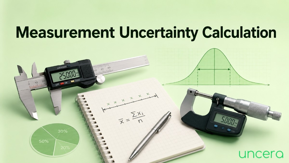
Calculate the mean. Add them up, divide by how many.

Calculate the standard deviation (s). Use the sample standard deviation, not the population one in Excel that’s STDEV.S, not STDEV.P. This trips people up regularly, and with small samples the difference is not small.

Divide by the square root of n:

u_A = s ÷ √n

That last step is the one students find odd. Why divide by √n? Because you’re not reporting a single reading you’re reporting the mean of your readings, and a mean is more reliable than any individual measurement. Take four times as many readings and this contribution halves.

It also tells you when to stop. Going from 5 readings to 10 buys you a 30% improvement. Going from 10 to 20 buys you another 30%. At some point the effort stops being worth it, and usually that point arrives sooner than people expect.

How to Calculate Uncertainty From a Single Reading

Sometimes you only get one shot, and there’s no standard deviation to work with. You can still assign an uncertainty.

Analogue instruments: half the smallest scale division. A steel rule marked in millimetres → ±0.5 mm. A dial gauge reading to 0.01 mm → ±0.005 mm.

Digital instruments: ±1 in the last displayed digit. A display reading 12.46 mm → ±0.01 mm.

Both of these give you the resolution uncertainty only, and it’s the floor, not the whole answer. If the instrument has a calibration certificate quoting something larger, use that instead. It usually will.

---

How to Calculate Percentage Uncertainty

Percentage uncertainty lets you compare measurements that have completely different units.

Percentage uncertainty = (absolute uncertainty ÷ measured value) × 100

25.002 ± 0.004 mm (0.004 ÷ 25.002) × 100 = 0.016%

Two things it’s useful for. First, comparing your instrument’s performance across different sizes the same micrometer gives a much worse percentage uncertainty on a 2 mm part than a 200 mm one. Second, propagating uncertainty through multiplication and division, which is the next section.

Divide by the value, not the uncertainty. It sounds obvious. It’s a surprisingly common slip under exam pressure.

---

How to Calculate Uncertainty When You Combine Measurements

You often measure two things and calculate a third. Each measurement drags its uncertainty into the result. Three rules cover almost everything:

Adding or subtracting → add the absolute uncertainties

12.5 ± 0.1 mm plus 8.3 ± 0.1 mm = 20.8 ± 0.2 mm

Note that subtracting doesn’t shrink the uncertainty. Uncertainties never cancel they only accumulate.

Multiplying or dividing → add the percentage uncertainties

Length 50.0 ± 0.1 mm (0.2%) × width 25.0 ± 0.1 mm (0.4%) Area = 1250 mm², combined 0.6% = 1250 ± 8 mm²

Powers and roots → multiply the percentage uncertainty by the power

Cube of side 20.0 ± 0.1 mm (0.5%) Volume = 8000 mm³, uncertainty 3 × 0.5% = 1.5% = 8000 ± 120 mm³

A square root counts as a power of ½, so it halves the percentage uncertainty.

These simple-addition rules are deliberately cautious. For independent sources, the statistically correct approach is quadrature √(0.2² + 0.4²) = 0.45% for the area example, rather than 0.6%. Coursework generally wants simple addition; professional work wants quadrature. Check which applies before you use it.

---

Common Mistakes When Calculating Uncertainty

Using population standard deviation instead of sample. STDEV.P instead of STDEV.S in Excel. With five readings the error is around 12%, and it always goes the wrong way it makes your uncertainty look smaller than it is.

Adding standard uncertainties directly instead of in quadrature. Squares first, then add, then square root. Straight addition inflates your uncertainty substantially and makes your measurement look worse than it is.

Forgetting to divide by √n in the Type A calculation. The standard deviation describes the spread of individual readings. You’re reporting a mean, and the mean is more reliable than any single reading.

Forgetting the divisors on Type B sources. Dropping a k=2 certificate value straight into the budget doubles that contribution. Convert everything to standard uncertainty first that’s the entire point of Step 4.

Mixing up resolution and half-resolution. For rectangular distributions you take half the resolution as the half-width, then divide by √3. Using the full resolution doubles the contribution.

Quoting uncertainty to four decimal places. ±0.003527 mm claims you know your doubt to four figures. You don’t. One significant figure, two at most.

Mismatched decimal places between value and uncertainty. 25.0024 ± 0.004 is inconsistent. Match them.

Omitting the coverage factor. ±0.004 mm could mean 68% or 95% confidence. Without k, the reader can’t tell, and the number is nearly useless.

Treating a known bias as uncertainty. If your certificate says the micrometer reads 0.002 mm high, correct for it. A known error should be removed, not absorbed into your uncertainty band.

Leaving out temperature. On anything long or precise, thermal effects are frequently the dominant term and they’re the one most often forgotten entirely.

---

Frequently Asked Questions

What is the formula to calculate uncertainty of measurement?

There are two. The combined standard uncertainty is u꜀ = √(u₁² + u₂² + …), where each u is a source expressed as a standard uncertainty. The expanded uncertainty is U = k × u꜀, where k is the coverage factor usually 2 for about 95% confidence.

How do you calculate Type A uncertainty?

Take repeated readings, calculate the sample standard deviation, then divide by the square root of the number of readings: u = s ÷ √n.

How do you calculate Type B uncertainty?

Take the value from a calibration certificate, manufacturer’s specification, resolution or published data, then divide by a factor based on its distribution 2 for a k=2 certificate, √3 for rectangular sources like resolution and tolerance limits.

Why do we divide by √3?

Because a rectangular distribution where the true value is equally likely anywhere between two limits has a standard deviation equal to its half-width divided by √3. It’s a property of the distribution, not an arbitrary choice.

Why combine uncertainties in quadrature instead of adding them?

Simple addition assumes every source goes wrong in the same direction simultaneously. Independent sources scatter randomly and partly cancel, and quadrature is the mathematically correct way to account for that.

What does k = 2 mean?

k is the coverage factor. Multiplying the combined standard uncertainty by 2 widens the interval from about 68% confidence to about 95%.

How many readings do I need?

Five as a minimum, ten if it’s quick. Because uncertainty falls as √n, the returns diminish fast going from 10 readings to 40 only halves the Type A contribution.

Can I calculate uncertainty from a single measurement?

Yes, but only Type B. Use half the smallest scale division for analogue instruments, or ±1 in the last digit for digital ones, plus any calibration certificate figure. You just won’t have a repeatability term.

Should uncertainty be reported to one or two significant figures?

One is standard for coursework. Many accredited laboratories use two throughout. Either works pick one and apply it consistently.

How small should my uncertainty be?

Small enough for the decision you’re making. A common guideline is no more than a quarter of the part’s tolerance. Beyond that you’re spending money for no benefit.

---

Conclusion

Calculating measurement uncertainty is bookkeeping with one unusual arithmetic rule. List your sources, put a number on each, convert them to the same units, combine in quadrature, multiply by two, round sensibly.

The parts worth remembering:

• Define the measurand first. It determines everything that follows.
• Type A comes from your readings (s ÷ √n). Type B comes from documents (divide by 2 for a k=2 certificate, by √3 for rectangular sources).
• Convert everything to standard uncertainty before combining. Skipping this step is the most common error in the whole process.
• Combine in quadrature, not by adding. Squares, sum, square root.
• Multiply by k = 2 for roughly 95% confidence, and always say so.
• Round the uncertainty to one significant figure, then match the value’s decimal places to it.

Every measurement you take is slightly wrong. Not because you are careless because no steel rule, micrometer or dial gauge in the world is perfect. Uncertainty is simply the honest way of saying how wrong your measurement might be.

The short answer: to find the uncertainty of a measurement, take half the smallest division on an analogue instrument, or ±1 in the last digit on a digital one. If you repeated the measurement, use half the range of your readings, or the standard deviation divided by √n. Then write your result as value ± uncertainty, with matching units.

That’s the summary. Below, we’ll unpack every part of it with worked examples you can copy straight into your lab report or inspection sheet.

What Is Measurement Uncertainty?

---

Measurement uncertainty is the range of values within which the true value of what you measured probably lies.

If you measure a shaft as 12.46 mm with a micrometer, you can’t honestly claim it is exactly 12.46 mm. What you can say is that it is somewhere around 12.46 mm probably within five microns either way. Writing it as 12.460 ± 0.005 mm communicates both the measurement and your confidence in it.

Every measurement result is incomplete without this second number. A reading on its own tells a reader what your instrument said. A reading with an uncertainty tells them how much to trust it which is exactly why every calibration certificate in the world carries one.

Uncertainty comes from a few places:

• The instrument — its resolution, and how well it was calibrated
• The method — operator feel on a micrometer thimble, parallax when reading a scale
• The part itself — a “round” shaft that is slightly out of roundness
• The environment — temperature drift, vibration, humidity

If you want the full picture of where uncertainty comes from and how labs quantify it formally, GaugeHow’s Uncertainty Measurement course walks through the complete process from basic terms to final calculation.

Uncertainty vs. Error vs. Accuracy vs. Precision

Students lose more marks and engineers lose more audit points confusing these four words than on almost anything else. Here’s the difference in one table:

Term	What it means	Can you calculate it?
Uncertainty	The range your true value probably sits in	Yes, from your own data
Error	The difference between your value and the true value	Only if the true value is known
Accuracy	How close your result is to the true value	Compare with the reference standard
Precision	How close your repeated readings are to each other	Look at the spread of your data

The key insight: uncertainty is not the same as error. Error requires knowing the right answer. Uncertainty is something you can work out from your measurements alone, without ever knowing the true value. That’s exactly why measurement professionals use it.

You can be precise but inaccurate five readings clustered tightly around the wrong number, because your micrometer has a zero error. And you can be accurate but imprecise readings scattered widely, but averaging out near the truth.

---

The Three Ways Uncertainty Is Written

The same uncertainty can be expressed three different ways. Exam questions and inspection reports switch between them constantly, so it’s worth being fluent in all three.

Absolute Uncertainty

The uncertainty written as a plain number, in the same units as your measurement.

12.460 ± 0.005 mm the absolute uncertainty is 0.005 mm.

Use it when you want to know the actual range of possible values.

Relative (Fractional) Uncertainty

The absolute uncertainty divided by the measured value. It has no units.

Relative uncertainty = absolute uncertainty ÷ measured value

0.005 ÷ 12.46 = 0.0004

Percentage Uncertainty

The relative uncertainty multiplied by 100.

Percentage uncertainty = (absolute uncertainty ÷ measured value) × 100

0.0004 × 100 = 0.04%

Percentage uncertainty is the most useful of the three, because it lets you compare measurements with completely different units. Is a ±0.005 mm uncertainty on a diameter worse than a ±0.2 °C uncertainty on a temperature? You can’t tell until you convert both to percentages.

---

How to Find Uncertainty From a Single Measurement

Most of the time you take one reading from one instrument. Here’s how to assign an uncertainty to it.

Analogue Instruments: Half the Smallest Division

For anything with a printed or graduated scale a steel rule, a vernier caliper, a micrometer, a dial gauge, a pressure gauge — the rule is:

Uncertainty = ½ × smallest scale division (least count)

The logic is simple. If a rule is marked every 1 mm, you can always tell which millimetre a length falls in. The most you could be out by is half of one of those gaps.

Instrument	Least count	Uncertainty
Steel rule	1 mm	±0.5 mm
Vernier caliper	0.02 mm	±0.01 mm
Outside micrometer	0.01 mm	±0.005 mm
Dial gauge	0.01 mm	±0.005 mm
Bourdon pressure gauge	0.5 bar	±0.25 bar
Thermometer	1 °C	±0.5 °C

Digital Instruments: ±1 in the Last Digit

A digital display can’t show you anything between its last two digits, so the uncertainty is one unit of that final decimal place.

Reading	Uncertainty
12.46 mm (digital caliper)	±0.01 mm
24.36 g	±0.01 g
0.818 V	±0.001 V

One caution, and it matters in industry: this is the resolution uncertainty only. If the instrument has a calibration certificate, or the manufacturer quotes a tolerance such as ±0.5% of reading, use that figure instead it will almost always be larger. Understanding how those certificate values are generated is the core of the Calibration Process (ISO/IEC 17025) course.

Worked Example: Measuring a Shaft With a Micrometer

You measure a shaft with an outside micrometer of least count 0.01 mm and read 12.46 mm.

1. Least count = 0.01 mm
2. Uncertainty = ½ × 0.01 mm = 0.005 mm
3. Result: 12.460 ± 0.005 mm
4. Percentage uncertainty = (0.005 ÷ 12.46) × 100 = 0.04%

A quick warning that catches people out: if you measure a length using both ends of a scale such as a steel rule, where you line up the zero mark and read the far end you are effectively taking two readings. Many methods double the uncertainty for this reason. Check what your course or procedure expects.

---

How to Find Uncertainty From Repeated Measurements

When you repeat a measurement several times, the spread of your readings tells you more than the instrument’s scale ever could. Two methods are standard.

Method 1: The Range Method

Fast, and accepted for most coursework and shop-floor checks.

Uncertainty = (largest reading − smallest reading) ÷ 2

Report the mean of your readings as the value, with this as the uncertainty.

Method 2: The Standard Deviation Method

More rigorous, and what accredited laboratories use. It’s officially called the standard uncertainty of the mean, or Type A uncertainty.

Uncertainty = s ÷ √n

Where s is the standard deviation of your readings and n is how many readings you took. Notice what this formula tells you: taking more readings shrinks your uncertainty, but only as √n. To halve your uncertainty you need four times as many measurements.

Worked Example: Five Readings on the Same Shaft

You measure the same shaft five times and record: 12.46, 12.48, 12.45, 12.47, 12.46 mm.

Step 1 — Find the mean: (12.46 + 12.48 + 12.45 + 12.47 + 12.46) ÷ 5 = 62.32 ÷ 5 = 12.464 mm

Step 2a — Range method: (12.48 − 12.45) ÷ 2 = 0.03 ÷ 2 = 0.015 mm → Result: 12.46 ± 0.02 mm

Step 2b — Standard deviation method: Standard deviation s = 0.011 mm Uncertainty = 0.011 ÷ √5 = 0.011 ÷ 2.24 = 0.005 mm → Result: 12.464 ± 0.005 mm

The standard deviation method gives a smaller uncertainty because it uses all five readings, not just the two extremes. Either is acceptable just state which one you used.

One thing repeating cannot fix: if your micrometer reads 0.02 mm with the anvils closed, every single reading is shifted the same way. Averaging won’t help. That’s a systematic error, and you have to find and remove it which is precisely what routine calibration and traceability to a reference standard exist to catch.

---

How to Combine Uncertainties When You Calculate Something

You rarely measure the quantity you actually want. You measure length and width, then calculate area. Each measurement carries uncertainty into the final answer this is called propagation of uncertainty, and it has three rules.

Rule 1: Adding or Subtracting → Add the ABSOLUTE Uncertainties

If y = a + b or y = a − b, then Δy = Δa + Δb

Two lengths: 12.5 ± 0.1 mm and 8.3 ± 0.1 mm Total length = 20.8 mm Uncertainty = 0.1 + 0.1 = 0.2 mm Result: 20.8 ± 0.2 mm

Note that the uncertainty grows even when you subtract. Uncertainties never cancel out they only accumulate.

Rule 2: Multiplying or Dividing → Add the PERCENTAGE Uncertainties

If y = a × b or y = a ÷ b, then %Δy = %Δa + %Δb

Plate length = 50.0 ± 0.1 mm → 0.2% Plate width = 25.0 ± 0.1 mm → 0.4% Area = 50.0 × 25.0 = 1250 mm² Percentage uncertainty = 0.2% + 0.4% = 0.6% Absolute uncertainty = 0.6% × 1250 = 7.5 mm² Result: 1250 ± 8 mm²

Rule 3: Powers and Roots → Multiply the Percentage Uncertainty by the Power

If y = aⁿ, then %Δy = n × %Δa

Cube of side 20.0 ± 0.1 mm → 0.5% Volume = 8000 mm³ Percentage uncertainty = 3 × 0.5% = 1.5% Absolute uncertainty = 1.5% × 8000 = 120 mm³ Result: 8000 ± 120 mm³

A square root counts as a power of ½, so it halves the percentage uncertainty.

A More Advanced Option: Adding in Quadrature

The rules above are deliberately cautious they assume every error pushes in the same unhelpful direction at once, which is unlikely. For independent random uncertainties, the statistically correct approach is to combine them in quadrature:

Combined % uncertainty = √( %Δa² + %Δb² + … )

For the plate example: √(0.2² + 0.4²) = 0.45%, rather than 0.6%. Most coursework wants the simple addition method; accredited laboratories and the GUM require quadrature. Check which applies to you before you use it.

---

Standard, Combined and Expanded Uncertainty

Once you move from coursework into real inspection and calibration work, three terms appear on every certificate:

• Standard uncertainty (u) — one contribution, expressed as one standard deviation. Roughly 68% confidence.
• Combined standard uncertainty (u_c) — all contributions merged in quadrature into a single figure.
• Expanded uncertainty (U) — the combined value multiplied by a coverage factor, usually k = 2, giving roughly 95% confidence.

U = k × u_c

So a certificate reading “±0.004 mm (k = 2)” means the combined standard uncertainty was about 0.002 mm, and the lab is 95% confident the true value falls inside that band.

Getting from a list of uncertainty sources to a defensible expanded uncertainty is the whole job of an uncertainty budget. GaugeHow covers budgets, coverage factors and confidence levels in the Uncertainty Measurement course, and the laboratory requirements behind them in the ISO/IEC 17025:2017 awareness programme.

---

How to Report Your Final Answer Correctly

Getting the number right and the formatting wrong still costs marks and fails audits. Four rules:

1. Round the uncertainty to one significant figure. 0.0387 becomes 0.04. The exception: if the first digit is a 1, keep two figures (0.134 → 0.13), because rounding to 0.1 would throw the value off too much.

2. Round the measurement to the same decimal place as the uncertainty. Writing 12.46384 ± 0.005 is meaningless. If you’re uncertain in the thousandths place, you cannot report hundred-thousandths. Write 12.464 ± 0.005.

3. Always include units on both numbers. 20.8 ± 0.2 mm, not 20.8 mm ± 0.2. Or factor the unit out: (20.8 ± 0.2) mm.

4. Say where the uncertainty came from. One line in your method “uncertainty taken as half the least count” shows the marker or auditor that you understand what you did.

---

The 7-Step Method (Quick Reference)

Use this as a checklist for any measurement task:

1. Define what you’re measuring and what you’ll calculate from it.
2. Take your measurements, repeating where practical.
3. Find the uncertainty in each individual measurement — least count, last digit, or spread of repeats.
4. Convert them all to percentage uncertainties so they can be compared.
5. Propagate them through your calculation using the add / multiply / power rules.
6. Convert back to an absolute uncertainty in the units of your final answer.
7. Round and report your result as value ± uncertainty, with units.

---

Common Mistakes When Calculating Uncertainty

These are the errors that show up again and again in marked reports and inspection records.

Quoting the uncertainty to too many significant figures. Writing ±0.00387 mm implies you know your uncertainty to three figures you don’t. One significant figure, almost always.

Mismatched decimal places. 12.46 ± 0.0015 mm is inconsistent: the value stops at hundredths but the uncertainty runs to ten-thousandths. Make them line up.

Adding percentages when you should add absolutes. Adding two lengths? Add the absolute uncertainties. Multiplying two lengths? Add the percentages. Getting this backwards is the single most common propagation mistake.

Confusing uncertainty with percentage error. Percentage error compares your result to a known reference value. Percentage uncertainty describes the spread in your own measurement. They are different quantities and often have very different values.

Dividing the range by the number of readings. The range method divides by 2, always not by n. It’s the standard deviation method that involves n.

Using the full least count instead of half. A rule marked in millimetres gives ±0.5 mm, not ±1 mm.

Assuming repeated measurements fix everything. Repeats reduce random uncertainty. A zero error or a drifted instrument survives any number of repeats untouched.

Ignoring the instrument’s calibration certificate. Resolution is only one contributor. If the certificate quotes a larger uncertainty, that’s the number you use.

Forgetting temperature. Steel expands roughly 11 µm per metre per °C. On a precision dimension measured outside 20 °C, this is often the largest single contributor and the one most often left out of the budget.

---

Frequently Asked Questions

What is the formula for uncertainty?

There isn’t one single formula. For a single reading from an analogue instrument, uncertainty = ½ × least count. For a digital instrument, it’s ±1 in the last digit displayed. For repeated readings, it’s either (max − min) ÷ 2 or the standard deviation divided by √n.

Is uncertainty the same as error?

No. Error is the difference between your measured value and the true value, which you can only calculate if you already know the true value. Uncertainty is the range your true value probably falls within, and you can work it out from your own measurements alone.

What is the uncertainty of a vernier caliper?

A vernier caliper with a least count of 0.02 mm gives ±0.01 mm from resolution alone. For any serious measurement, check the calibration certificate the certified uncertainty is usually larger.

How many readings should I take?

Three is a minimum; five or more is better. Because uncertainty falls as √n, the improvement slows quickly going from 5 readings to 20 only halves your uncertainty.

What does ±2% uncertainty mean?

It means the true value probably lies within 2% either side of your measured value. A reading of 50.0 mm with 2% uncertainty means the true dimension is likely between 49.0 mm and 51.0 mm.

Can uncertainty ever be zero?

No. Every measurement has some uncertainty. Counted quantities 12 parts, 5 trials are exact, but those aren’t measurements. If you calculate an uncertainty of zero, something has gone wrong in your method.

What’s the difference between standard and expanded uncertainty?

Standard uncertainty is roughly one standard deviation, covering about 68% of likely values. Expanded uncertainty multiplies it by a coverage factor usually k = 2 to give roughly 95% confidence. Calibration laboratories report expanded uncertainty; students usually report standard uncertainty.

Do I need to include uncertainty in every report?

Yes, for any quantitative result. A measurement without a stated uncertainty is an incomplete result, and ISO/IEC 17025 requires accredited laboratories to evaluate and report it.

---

Key Takeaways

• Uncertainty tells your reader how much to trust a measurement it is not a mistake or a failure.
• Single reading: half the least count (analogue) or ±1 in the last digit (digital).
• Repeated readings: half the range, or standard deviation ÷ √n.
• Adding or subtracting → add absolute uncertainties. Multiplying or dividing → add percentage uncertainties. Powers → multiply the percentage by the power.
• Expanded uncertainty = combined standard uncertainty × coverage factor, usually k = 2.
• Round the uncertainty to one significant figure, then match your value’s decimal places to it.

Ask ten students to measure the same wire with the same vernier caliper, and you’ll get several different answers. Nobody has done anything wrong. That’s just what measurement is.

Physics deals with this honestly. Instead of pretending a reading is exact, we state a range: the value, plus how far off it might be. That range is the uncertainty, and every experimental result in physics carries one.

This guide covers everything you need for a physics lab report or an exam question: least count, absolute and percentage error, the propagation rules, significant figures, and worked numericals you can follow line by line.

---

What Is Uncertainty in Measurement?

Uncertainty in measurement is the range of values within which the true value of a physical quantity is likely to lie.

When you write a length as 2.64 ± 0.01 cm, you’re making two statements at once. Your best estimate is 2.64 cm. And the true length is probably somewhere between 2.63 and 2.65 cm.

Without that second number, the first one is incomplete. A reading on its own tells your teacher what the instrument said. A reading with an uncertainty tells them how much to trust it and in physics, that’s the whole point of doing the experiment carefully.

A quick note on wording, because it confuses people: your physics textbook probably says error where a metrology handbook would say uncertainty. In NCERT and most school syllabuses you’ll meet absolute error, mean absolute error, relative error and percentage error. They’re describing the same idea. Don’t let the vocabulary throw you.

---

Why Every Physical Measurement Has Uncertainty

Uncertainty isn’t a sign of carelessness. It’s built into the act of measuring. Four reasons:

The instrument can only resolve so much. A metre scale marked in millimetres cannot tell you where something falls within a millimetre. That limit has a name the least count and it never goes away, no matter how carefully you look.

Your senses and reflexes are limited. Starting and stopping a stopwatch involves reaction time of roughly 0.2 seconds. Judging when a pointer sits exactly on a mark involves eyesight and angle.

Conditions change. Temperature affects the length of a metal rod. Air currents affect a sensitive balance. Voltage fluctuations affect a circuit.

The quantity itself isn’t perfectly defined. A “uniform” wire is slightly thicker at one end. A “spherical” ball bearing is slightly out of round. Where you measure changes what you get.

Add these up and you get scatter. Uncertainty is simply the number that describes that scatter honestly.

---

Errors and Uncertainty: What’s the Difference?

These two words are used loosely in the lab and precisely in exams, so it’s worth pinning down.

Error is the difference between your measured value and the true value. To calculate it, you have to know the true value — which you usually don’t, though in sch ool experiments you often have a standard value to compare against (g = 9.8 m/s², for instance).

Uncertainty is the range in which the true value probably sits. You work it out from your own readings and your instrument, without ever needing to know the right answer.

That’s the key practical difference. You can always state an uncertainty. You can only state an error when someone has already told you the answer.

Two related words that get muddled with them:

Accuracy how close your result is to the true value. Precision how close your repeated readings are to each other.

You can be precise but inaccurate. Five stopwatch readings all within 0.02 s of each other, taken with a stopwatch that runs slow, are beautifully precise and consistently wrong. Repeating a measurement can never reveal that kind of fault.

---

Types of Errors in Measurement

Physics syllabuses classify errors by cause. Three categories:

Systematic Errors

These shift every reading in the same direction by roughly the same amount. Repeating the measurement won’t help — the error just comes along for the ride.

Common ones in a school lab:

• Zero error — a vernier caliper that reads 0.02 cm when the jaws are closed, or a screw gauge with a zero offset
• Instrumental error — a stopwatch running slow, an ammeter poorly calibrated
• Imperfect technique — reading a scale from an angle every time (parallax), or not letting a thermometer settle
• Personal bias — consistently stopping the timer a fraction early

The good news: systematic errors can be found and corrected. Check for zero error before you start. Read scales straight on. Calibrate against a known standard.

Random Errors

These scatter your readings unpredictably sometimes high, sometimes low. Reaction time on a stopwatch, small fluctuations in temperature, tiny variations in how hard you tighten a screw gauge.

Random errors can be reduced by taking more readings and averaging, because the high ones and low ones partly cancel out.

Gross Errors

Plain mistakes. Misreading 2.64 as 2.46. Writing down the wrong unit. Forgetting to add the vernier scale reading to the main scale reading.

These aren’t uncertainty and you don’t include them in a calculation. You find them and fix them. If one reading in a set is wildly out of line with the others, check your working before you average it in.

---

Least Count and Instrument Uncertainty

The least count of an instrument is the smallest value it can measure the size of one division on its scale.

Instrument	Least count
Metre scale	0.1 cm (1 mm)
Vernier caliper	0.01 cm (0.1 mm)
Screw gauge / micrometer	0.001 cm (0.01 mm)
Spherometer	0.001 cm
Stopwatch (digital)	0.01 s
Stopwatch (analogue)	0.1 s or 1 s
Laboratory thermometer	1 °C

For a vernier caliper you calculate it yourself:

Least count = value of 1 main scale division ÷ number of vernier scale divisions

1 MSD = 1 mm, 10 vernier divisions LC = 1 ÷ 10 = 0.1 mm = 0.01 cm

For a screw gauge:

Least count = pitch ÷ number of circular scale divisions

Pitch = 1 mm, 100 circular divisions LC = 1 ÷ 100 = 0.01 mm = 0.001 cm

The least count sets the floor on your uncertainty. You cannot be more certain than your instrument can resolve.

---

How to Find Uncertainty From a Single Reading

When you take one reading and can’t repeat it, the uncertainty comes from the instrument itself.

Analogue instruments half the least count. A metre scale with 1 mm divisions gives ±0.5 mm. The logic: you can always tell which millimetre a length falls in, so the most you can be out by is half a division.

Digital instruments ±1 in the last digit. A digital stopwatch showing 12.46 s gives ±0.01 s.

Vernier calipers and screw gauges usually the full least count. Most physics syllabuses take the uncertainty as ± the least count for these, not half of it, because the vernier scale is already designed to resolve to that level. So a vernier caliper gives ±0.01 cm and a screw gauge ±0.001 cm.

That last convention varies between boards and textbooks, so check which one your syllabus uses before an exam. Whichever you pick, state it in your report.

One more trap. If you measure a length by lining up the zero of a metre scale at one end and reading the other end, that’s two readings both ends carry uncertainty. Some methods double the uncertainty to account for this.

---

How to Find Uncertainty From Repeated Readings

Take a measurement several times and the spread of your readings tells you more than the least count ever could. Here’s the standard physics method.

Step 1 — Find the mean.

a_mean = (a₁ + a₂ + … + aₙ) ÷ n

Step 2 — Find the absolute error in each reading. This is how far each reading sits from the mean, ignoring the sign.

Δaᵢ = |a_mean − aᵢ|

Step 3 — Find the mean absolute error. Average those.

Δa_mean = (Δa₁ + Δa₂ + … + Δaₙ) ÷ n

Step 4 — Report the result.

a = a_mean ± Δa_mean

Solved Example

You measure a rod five times with a vernier caliper: 2.63, 2.65, 2.64, 2.62, 2.66 cm.

Mean: (2.63 + 2.65 + 2.64 + 2.62 + 2.66) ÷ 5 = 13.20 ÷ 5 = 2.640 cm

Absolute errors: |2.640 − 2.63| = 0.010 |2.640 − 2.65| = 0.010 |2.640 − 2.64| = 0.000 |2.640 − 2.62| = 0.020 |2.640 − 2.66| = 0.020

Mean absolute error: (0.010 + 0.010 + 0.000 + 0.020 + 0.020) ÷ 5 = 0.060 ÷ 5 = 0.012 cm

Result: 2.64 ± 0.01 cm

Notice the mean absolute error (0.012 cm) came out larger than the least count (0.01 cm). When that happens, use the larger figure your readings are telling you the real scatter is bigger than the instrument’s resolution.

---

Absolute, Relative and Percentage Uncertainty

The same uncertainty gets written three ways, and questions switch between them constantly.

Absolute error (Δa) — a plain number in the same units as the measurement.

2.64 ± 0.01 cm

Relative error — the absolute error divided by the mean value. No units.

Relative error = Δa_mean ÷ a_mean 0.012 ÷ 2.640 = 0.0045

Percentage error — relative error × 100.

Percentage error = (Δa_mean ÷ a_mean) × 100 0.0045 × 100 = 0.45%

Percentage error is the most useful of the three, for one reason: it lets you compare measurements with different units. Is ±0.01 cm on a length worse than ±0.1 s on a time? You can’t tell until both are percentages.

It also tells you which measurement is dragging your experiment down. That turns out to matter a lot, as the pendulum example below shows.

---

Combination of Errors: The Propagation Rules

You rarely measure the quantity you actually want. You measure length and time, then calculate g. You measure mass and volume, then calculate density. Each measurement carries its uncertainty into the final answer.

Four rules cover almost every physics numerical.

Rule 1 — Sum or Difference: Add the Absolute Errors

If Z = A + B or Z = A − B, then ΔZ = ΔA + ΔB

A = 12.5 ± 0.1 cm, B = 8.3 ± 0.1 cm A + B = 20.8 ± 0.2 cm A − B = 4.2 ± 0.2 cm

Look at that second line carefully. The uncertainty is the same whether you add or subtract, but the value got much smaller so the percentage error shot up from 1% to nearly 5%. Subtracting two similar numbers is the fastest way to wreck an experiment’s precision. Design your method to avoid it where you can.

Rule 2 — Product or Quotient: Add the Relative Errors

If Z = A × B or Z = A ÷ B, then ΔZ/Z = ΔA/A + ΔB/B

Mass m = 5.74 ± 0.01 g → 0.17% Volume V = 1.2 ± 0.1 cm³ → 8.3% Density ρ = 5.74 ÷ 1.2 = 4.783 g/cm³ Δρ/ρ = 0.17% + 8.3% = 8.5% Δρ = 0.085 × 4.783 = 0.41 ρ = 4.8 ± 0.4 g/cm³

The volume measurement contributes almost all the uncertainty. Weighing the sample more precisely would be pointless — you’d need a better way to measure volume.

Rule 3 — Powers: Multiply the Relative Error by the Power

If Z = Aⁿ, then ΔZ/Z = n × (ΔA/A)

Side of a cube = 20.0 ± 0.1 mm → 0.5% Volume = 8000 mm³ Relative error = 3 × 0.5% = 1.5% ΔV = 0.015 × 8000 = 120 mm³ V = 8000 ± 120 mm³

A square root is a power of ½, so it halves the relative error.

Rule 4 — The General Formula

For anything of the form Z = AᵖBᑫ / Cʳ:

ΔZ/Z = p(ΔA/A) + q(ΔB/B) + r(ΔC/C)

Every power counts, and every term is added — never subtracted, even when the quantity appears in the denominator. Uncertainties only accumulate.

---

Solved Example: Finding g With a Simple Pendulum

This is the classic, and it shows exactly why the propagation rules matter.

The formula: T = 2π√(L/g), rearranged to g = 4π²L / T²

Applying Rule 4:

Δg/g = ΔL/L + 2(ΔT/T)

Note the 2 on the time term. T is squared in the formula, so its relative error counts double.

Your measurements:

• Length of pendulum, metre scale: L = 100.0 ± 0.1 cm
• Time for 20 oscillations, stopwatch: t = 40.0 ± 0.1 s

Find T: T = 40.0 ÷ 20 = 2.00 s ΔT = 0.1 ÷ 20 = 0.005 s

Calculate g: g = 4π² × 1.000 ÷ (2.00)² = 9.87 m/s²

Propagate the uncertainty: ΔL/L = 0.1 ÷ 100.0 = 0.001 → 0.1% 2(ΔT/T) = 2 × (0.005 ÷ 2.00) = 0.005 → 0.5% Δg/g = 0.1% + 0.5% = 0.6%

Absolute uncertainty: Δg = 0.006 × 9.87 = 0.059 ≈ 0.06

Result: g = 9.87 ± 0.06 m/s²

The lesson hiding in that example

Timing contributed 0.5% of the 0.6% total. Length contributed 0.1%. Measuring the pendulum length more carefully would barely change the answer.

But time 100 oscillations instead of 20 and Δt stays 0.1 s while t becomes 200 s. Now ΔT = 0.001 s, and the time contribution drops to 0.1%. Your total uncertainty falls from 0.6% to 0.2% a threefold improvement, for free, just by counting more swings.

That’s what error analysis is actually for. Not the number at the end. Finding out which measurement is hurting you, so you know where to put your effort.

---

Uncertainty and Significant Figures

Significant figures aren’t a separate topic. They’re how you communicate uncertainty when you haven’t written a ± explicitly.

Writing 9.87 m/s² implies you’re confident to the second decimal place. Writing 9.87456 m/s² claims you know it to five decimals and if your uncertainty is ±0.06, that’s simply false.

Three rules for reporting:

Round the uncertainty to one significant figure. 0.059 becomes 0.06. The one exception: if the leading digit is 1, keep two figures (0.134 → 0.13), since rounding to 0.1 would distort it badly.

Round the value to match the uncertainty’s decimal place. If your uncertainty stops at the second decimal, so does your value. 9.87456 ± 0.06 becomes 9.87 ± 0.06.

Put units on both numbers, or factor them out: (9.87 ± 0.06) m/s².

Two more that matter in calculations:

• In addition and subtraction, the answer keeps the fewest decimal places of any input.
• In multiplication and division, the answer keeps the fewest significant figures of any input.

Keep extra digits during intermediate steps and round only at the end. Rounding halfway through introduces errors that have nothing to do with your measurements.

---

Uncertainty in Graphs and Error Bars

Most physics experiments end in a graph, and the gradient usually is the answer. So your gradient needs an uncertainty too.

Error bars show the uncertainty on each plotted point a vertical line extending ±Δy above and below, and a horizontal one for ±Δx. If the uncertainty is too small to see at your scale, say so in the report rather than leaving them off silently.

Finding the uncertainty in the gradient:

1. Draw the line of best fit through your points and calculate its gradient, m.
2. Draw the steepest reasonable line that still passes through all the error bars. Find its gradient, m_max.
3. Draw the shallowest reasonable line that does the same. Find m_min.
4. Δm = (m_max − m_min) ÷ 2

Report the gradient as m ± Δm.

The same method works for the y-intercept. And the width of the gap between your steepest and shallowest lines tells you something immediately: if it’s large, your data is scattered and your conclusion is weak, however neat the best-fit line looks on its own.

---

How to Reduce Uncertainty in a Physics Experiment

Work down this list in order the first three are worth more than the rest combined.

1. Find your dominant source first. Convert everything to percentages and see which one is biggest. Improving anything else is wasted effort. This single habit separates good lab reports from average ones.

2. Measure many, divide by many. Time 100 oscillations instead of 10. Measure the thickness of 50 sheets of paper and divide by 50. Your instrument’s uncertainty gets divided by the count while the quantity stays the same. It’s the highest-leverage trick in experimental physics.

3. Repeat and average. Random errors partly cancel. Five readings minimum, more if they’re quick.

4. Check for zero error before you start. Close the caliper jaws. Look at the reading. Note it and subtract it. This takes five seconds and fixes a systematic error that averaging can never touch.

5. Use an instrument with a smaller least count. A screw gauge instead of a vernier caliper is a tenfold improvement but only if the least count is actually your limiting factor.

6. Avoid subtracting similar quantities. As Rule 1 showed, this inflates percentage error dramatically. Redesign the method if you can.

7. Kill parallax. Read scales straight on, with your eye level with the mark. Use a mirror scale if the apparatus has one.

8. Control the conditions. Shield a sensitive balance from draughts. Let apparatus reach room temperature before measuring.

---

Common Mistakes Students Make

Writing a result with no uncertainty at all. An experimental value without a ± is incomplete, and most mark schemes allocate points specifically for it.

Quoting the uncertainty to three or four figures. ±0.0592 m/s² claims you know your doubt to three significant figures. You don’t. Round to one.

Mismatched decimal places. 9.8 ± 0.06 is inconsistent the value stops at tenths but the uncertainty runs to hundredths. Line them up.

Adding percentages when you should add absolutes. Adding two lengths? Add the absolute errors. Multiplying them? Add the relative errors. Getting this backwards is the single most common propagation mistake in exams.

Forgetting the power in the propagation rule. In g = 4π²L/T², the T term must be multiplied by 2. Miss it and your uncertainty comes out almost half what it should be.

Dividing the mean absolute error by the wrong thing. For relative error you divide by the mean value, not by n and not by the least count.

Assuming repeating readings fixes everything. Repeats reduce random error only. A zero error survives any number of repeats untouched.

Ignoring the least count when the scatter is small. If your five readings are identical, your mean absolute error is zero — but your uncertainty isn’t. Fall back on the least count.

Confusing percentage error with percentage difference from the standard value. Percentage error describes the spread in your own measurement. Comparing your g to 9.8 m/s² is a different calculation with a different name.

Dropping units. ±0.06 means nothing on its own.

---

Frequently Asked Questions

What is uncertainty in measurement in physics?

It’s the range of values within which the true value of a measured quantity is likely to lie. It’s reported alongside the measurement, as value ± uncertainty, and every experimental result in physics has one.

What is the difference between error and uncertainty?

Error is the difference between your measured value and the true value, so you need the true value to calculate it. Uncertainty is the range the true value probably falls within, and you work it out from your own readings.

What is the formula for absolute error?

Δaᵢ = |a_mean − aᵢ| for each reading. The mean absolute error is the average of those values: Δa_mean = Σ|Δaᵢ| ÷ n.

What is the formula for percentage error?

Percentage error = (mean absolute error ÷ mean value) × 100.

What is the least count of a vernier caliper?

For a standard vernier caliper with 10 vernier divisions matching 9 main scale divisions of 1 mm each, the least count is 0.1 mm, which is 0.01 cm. Calculate it as: 1 main scale division ÷ number of vernier divisions.

How do you combine uncertainties in physics?

For sums and differences, add the absolute errors. For products and quotients, add the relative errors. For powers, multiply the relative error by the power. All terms are added, never subtracted.

Why do we multiply by 2 in the pendulum uncertainty formula?

Because T appears squared in g = 4π²L/T². Under the propagation rules, a quantity raised to the power n contributes n times its relative error — so T² contributes twice.

How many readings should I take in a physics experiment?

Three is the usual minimum for school experiments, five is better. Beyond about ten the improvement becomes small compared with the extra effort.

Can uncertainty ever be zero?

No. Every measurement has some. If your repeated readings are all identical, your uncertainty isn’t zero — it’s the least count of your instrument.

Do I need to show uncertainty in every lab report?

Yes, for every quantitative result. It’s usually worth marks on its own, and a result without it is treated as incomplete.

---

Conclusion

Uncertainty in measurement isn’t an admission that your experiment went badly. It’s what turns a number into a scientific result.

The essentials to carry into your next lab session:

• Uncertainty is the range the true value probably lies in. It’s never zero, and it’s not the same as error.
• Single reading? Use half the least count for analogue scales, ±1 in the last digit for digital, and the full least count for vernier calipers and screw gauges (check your syllabus).
• Repeated readings? Find the mean, then the mean absolute error. If it comes out smaller than the least count, use the least count instead.
• Percentage error = (absolute error ÷ mean value) × 100. Convert everything to percentages so you can compare across units.
• Propagation: add absolute errors for sums and differences, relative errors for products and quotients, and multiply by the power for exponents.
• Round the uncertainty to one significant figure, then match your value’s decimal places to it.

Most people arriving here don’t want a lecture. They want the formula, the symbols explained, and a worked number to check their spreadsheet against.

So that’s what this page is — every uncertainty formula you’ll need, grouped by what it does, with a full formula sheet near the bottom you can screenshot.

---

The Two Formulas That Matter Most

If you only remember two, make it these.

Combined standard uncertainty

u꜀ = √(u₁² + u₂² + u₃² + … + uₙ²)

Expanded uncertainty

U = k × u꜀

Everything else on this page either feeds numbers into the first formula or interprets what comes out of the second.

---

Symbols Used in Uncertainty Formulas

Half the confusion with these formulas is notation. Here’s the key.

Symbol	Meaning
x̄	Mean of your readings
s	Sample standard deviation
n	Number of readings taken
u	Standard uncertainty of one source
u(xᵢ)	Standard uncertainty of input quantity i
u꜀	Combined standard uncertainty
U	Expanded uncertainty
k	Coverage factor (usually 2)
cᵢ	Sensitivity coefficient for input i
a	Half-width of a rectangular distribution
ν	Degrees of freedom
ν_eff	Effective degrees of freedom
α	Coefficient of thermal expansion

One convention worth noting: lower-case u is always a standard uncertainty (roughly 68% confidence). Upper-case U is always expanded (roughly 95%). Mixing them up is the most common notation error in the whole subject.

---

Formula for Type A Uncertainty

Type A uncertainty is calculated statistically, from repeated readings.

Mean:

x̄ = (x₁ + x₂ + … + xₙ) ÷ n

Sample standard deviation:

s = √[ Σ(xᵢ − x̄)² ÷ (n − 1) ]

Type A standard uncertainty:

u_A = s ÷ √n

The divisor in the standard deviation formula is n − 1, not n. In Excel that means STDEV.S, not STDEV.P. With small samples the difference is significant and it always makes your uncertainty look smaller than it really is.

The √n in the last step is there because you’re reporting the mean of your readings, not any single one, and a mean is more reliable than an individual measurement.

---

Formula for Type B Uncertainty

Type B uncertainty comes from certificates, specifications and published data rather than from repeating the measurement. Each source is converted to a standard uncertainty by dividing by a factor that depends on its assumed distribution.

General form:

u_B = a ÷ divisor

Where a is the half-width of the interval.

Source of the number	Distribution	Formula
Certificate stating k = 2	Normal	u = U ÷ 2
Certificate stating k = 3	Normal	u = U ÷ 3
Resolution of an instrument	Rectangular	u = a ÷ √3
Manufacturer’s ± limits	Rectangular	u = a ÷ √3
Temperature between two limits	Rectangular	u = a ÷ √3
Value most likely near the centre	Triangular	u = a ÷ √6
Value most likely near the extremes	U-shaped	u = a ÷ √2

Resolution specifically:

u = (resolution ÷ 2) ÷ √3 = resolution ÷ (2√3) ≈ resolution × 0.289

That shortcut is worth memorising. A 0.01 mm resolution gives 0.01 × 0.289 = 0.0029 mm.

When you have limits and nothing else, use rectangular. It’s the conservative assumption and the one the GUM recommends by default.

---

Formula for Sensitivity Coefficients

A sensitivity coefficient converts an input’s uncertainty into the units of your result, and scales it by how strongly it affects the outcome.

General form:

cᵢ = ∂f / ∂xᵢ

That’s the partial derivative of your measurement equation with respect to that input. In practice you rarely differentiate anything:

• Direct measurements (micrometer on a shaft): c = 1
• Thermal expansion: c = L × α
• A quantity that appears squared: c effectively doubles its relative contribution

Thermal example:

c = L × α = 25 mm × 11.5 × 10⁻⁶ /°C = 0.000288 mm/°C

Contribution to the budget:

uᵢ(y) = cᵢ × u(xᵢ)

---

Formula for Combined Standard Uncertainty

Once every source is a standard uncertainty in the same units, combine them.

Simple form (all sensitivity coefficients = 1):

u꜀ = √(u₁² + u₂² + … + uₙ²)

With sensitivity coefficients:

u꜀ = √[ Σ (cᵢ · u(xᵢ))² ]

Full GUM law of propagation:

u꜀²(y) = Σ (∂f/∂xᵢ)² · u²(xᵢ)

All three say the same thing at increasing levels of formality: square each contribution, add the squares, take the square root.

This is called adding in quadrature. Straight addition would assume every source goes wrong in the same direction at the same instant — possible, but unlikely for independent sources.

Note on correlation. These formulas assume the sources are independent. If two share a common cause, a covariance term is strictly required:

u꜀² = Σ cᵢ² u²(xᵢ) + 2 ΣΣ cᵢ cⱼ u(xᵢ, xⱼ)

Routine work usually ignores it. Just know it exists.

---

Formula for Expanded Uncertainty

U = k × u꜀

k	Approximate confidence
1	68.27%
2	95.45%
2.58	99%
3	99.73%

k = 2 is the default. Use it unless a customer, standard or examiner specifies otherwise. Always state the value of k next to the result — “±0.010 mm” without it is an incomplete statement.

---

Formula for Absolute, Relative and Percentage Uncertainty

Three ways of expressing the same thing.

Absolute uncertainty — a number in the units of the measurement.

50.020 ± 0.010 mm → absolute uncertainty = 0.010 mm

Relative uncertainty

Relative uncertainty = Δx ÷ x 0.010 ÷ 50.020 = 0.0002

Percentage uncertainty

Percentage uncertainty = (Δx ÷ x) × 100 0.0002 × 100 = 0.020%

Divide by the measured value, not by the uncertainty. It sounds too obvious to mention, and it’s still one of the most frequent slips under exam conditions.

---

Uncertainty Propagation Formulas

When you calculate a result from two or more measurements, their uncertainties propagate through. Two versions of each rule exist — the simple arithmetic form used in most coursework, and the quadrature form used in professional work.

Sum or Difference: Z = A ± B

Simple: ΔZ = ΔA + ΔB Quadrature: ΔZ = √(ΔA² + ΔB²)

Add the absolute uncertainties. This holds for subtraction too — uncertainties never cancel.

Product or Quotient: Z = A × B or A ÷ B

Simple: ΔZ/Z = ΔA/A + ΔB/B Quadrature: ΔZ/Z = √[(ΔA/A)² + (ΔB/B)²]

Add the relative uncertainties.

Powers: Z = Aⁿ

ΔZ/Z = n × (ΔA/A)

A square root is a power of ½, so it halves the relative uncertainty.

General Form: Z = Aᵖ · Bᑫ ÷ Cʳ

Simple: ΔZ/Z = p(ΔA/A) + q(ΔB/B) + r(ΔC/C) Quadrature: ΔZ/Z = √[ p²(ΔA/A)² + q²(ΔB/B)² + r²(ΔC/C)² ]

Every term is added, including the ones in the denominator. There are no minus signs in uncertainty propagation.

---

Formula for Uncertainty From Least Count

When you take a single reading and have no repeats to work with, the instrument sets the uncertainty.

Analogue instruments: u = least count ÷ 2 Digital instruments: u = ±1 in the last displayed digit Vernier caliper / screw gauge (physics convention): u = least count

Least count formulas:

Vernier caliper: LC = 1 main scale division ÷ number of vernier divisions Screw gauge: LC = pitch ÷ number of circular scale divisions

Example: pitch 1 mm, 100 circular divisions → LC = 0.01 mm

The half-least-count versus full-least-count convention for vernier instruments varies between syllabuses and standards. Check which applies to you, then state it in your report.

---

Formula for Mean Absolute Error

Physics courses often use this instead of standard deviation. Same purpose, simpler arithmetic.

Mean: a_mean = (a₁ + a₂ + … + aₙ) ÷ n Absolute error of each reading: Δaᵢ = |a_mean − aᵢ| Mean absolute error: Δa_mean = (Δa₁ + Δa₂ + … + Δaₙ) ÷ n Relative error: Δa_mean ÷ a_mean Percentage error: (Δa_mean ÷ a_mean) × 100

Result reported as a_mean ± Δa_mean.

If the mean absolute error comes out smaller than the instrument’s least count, use the least count instead. Your readings can’t be more certain than your instrument can resolve.

---

Degrees of Freedom and the Welch–Satterthwaite Formula

This is where k = 2 stops being automatic. If your Type A uncertainty is based on very few readings, k = 2 doesn’t actually deliver 95% confidence — you need a larger factor.

Degrees of freedom:

Type A: ν = n − 1 Type B: ν = ∞ (assumed, when the source is well characterised)

Welch–Satterthwaite formula for effective degrees of freedom:

ν_eff = u꜀⁴ ÷ Σ (uᵢ⁴ ÷ νᵢ)

Coverage factor from ν_eff (t-distribution, ~95.45% confidence):

ν_eff	k
1	13.97
2	4.53
3	3.31
4	2.87
5	2.65
6	2.52
8	2.37
10	2.28
20	2.13
50	2.05
∞	2.00

In most real budgets the Type B sources dominate and ν_eff comes out large, so k = 2 is fine. It matters when repeatability is your biggest term and you only took three or four readings — then k = 2 quietly understates your uncertainty.

---

The Complete Formula Sheet

Everything above, in one place.

What you need	Formula
Mean	x̄ = Σxᵢ ÷ n
Sample standard deviation	s = √[Σ(xᵢ − x̄)² ÷ (n−1)]
Type A uncertainty	u_A = s ÷ √n
Type B — from k=2 certificate	u = U ÷ 2
Type B — rectangular	u = a ÷ √3
Type B — triangular	u = a ÷ √6
Type B — resolution	u ≈ resolution × 0.289
Sensitivity coefficient	cᵢ = ∂f/∂xᵢ
Thermal sensitivity	c = L × α
Combined standard uncertainty	u꜀ = √[Σ(cᵢuᵢ)²]
Expanded uncertainty	U = k × u꜀
Relative uncertainty	Δx ÷ x
Percentage uncertainty	(Δx ÷ x) × 100
Propagation — sum/difference	ΔZ = ΔA + ΔB
Propagation — product/quotient	ΔZ/Z = ΔA/A + ΔB/B
Propagation — power	ΔZ/Z = n(ΔA/A)
Least count — vernier	LC = MSD ÷ no. of vernier divisions
Least count — screw gauge	LC = pitch ÷ circular divisions
Uncertainty from analogue scale	u = LC ÷ 2
Mean absolute error	Δa = Σ|a_mean − aᵢ| ÷ n
Effective degrees of freedom	ν_eff = u꜀⁴ ÷ Σ(uᵢ⁴ ÷ νᵢ)

---

Which Formula Do You Need?

A quick decision path.

Did you take repeated readings? → Yes: u_A = s ÷ √n → No: use the least count formula

Do you have a calibration certificate? → Divide its stated U by the k value printed on it

Do you have a manufacturer’s tolerance or a resolution figure? → Divide the half-width by √3

Do you have several sources to merge? → u꜀ = √(Σuᵢ²)

Do you need a confidence level for reporting? → U = 2 × u꜀

Are you calculating one quantity from several measurements? → Use the propagation rules

Is your repeatability the dominant term and n is small? → Check ν_eff and use the t-table instead of assuming k = 2

---

Worked Example Using the Formulas

A digital caliper measuring a 50 mm gauge block.

Readings: 50.02, 50.03, 50.01, 50.02, 50.02 mm

Mean: x̄ = 250.10 ÷ 5 = 50.020 mm

Standard deviation: s = 0.0071 mm

Type A: u_A = 0.0071 ÷ √5 = 0.0032 mm

Type B — resolution (0.01 mm): u = 0.01 × 0.289 = 0.0029 mm

Type B — calibration certificate, U = 0.004 mm at k = 2: u = 0.004 ÷ 2 = 0.0020 mm

Combined: u꜀ = √(0.0032² + 0.0029² + 0.0020²) = √(0.0000226) = 0.0048 mm

Check the degrees of freedom: ν_A = 5 − 1 = 4, ν_B = ∞ ν_eff = (0.0048)⁴ ÷ [(0.0032)⁴ ÷ 4] ≈ 20 From the table, ν_eff = 20 gives k = 2.13 — close enough to 2 that it makes no practical difference here.

Expanded: U = 2 × 0.0048 = 0.0096 ≈ 0.010 mm

Result: 50.020 ± 0.010 mm (k = 2, approximately 95% confidence)

Percentage uncertainty: (0.010 ÷ 50.020) × 100 = 0.020%

---

Common Mistakes When Applying These Formulas

Using population standard deviation. STDEV.P divides by n instead of n−1. With five readings that understates your uncertainty by about 12%.

Forgetting √n in the Type A formula. The standard deviation describes individual readings. You’re reporting a mean, which is more reliable.

Dropping a certificate value straight into the budget. A k = 2 figure must be divided by 2 first. Skipping that step doubles the contribution.

Adding standard uncertainties instead of combining in quadrature. Squares, sum, square root. Straight addition inflates the total substantially.

Using the full resolution as the half-width. For rectangular sources, a is half the resolution, then divide by √3.

Confusing u and U. Lower case is standard, upper case is expanded. They differ by a factor of 2.

Mixing absolute and relative in propagation. Sums and differences use absolute. Products and quotients use relative. Getting this backwards is the classic exam error.

Missing the exponent in the power rule. In g = 4π²L/T², the T term is multiplied by 2 because T is squared.

Assuming k = 2 with very few readings. If repeatability dominates and n is small, run Welch–Satterthwaite and read k from the t-table.

Reporting without stating k. The number is ambiguous without it.

---

Frequently Asked Questions

What is the formula for uncertainty of measurement? The two core formulas are the combined standard uncertainty, u꜀ = √(u₁² + u₂² + …), and the expanded uncertainty, U = k × u꜀, where k is normally 2 for about 95% confidence.

What is the formula for Type A uncertainty? u_A = s ÷ √n, where s is the sample standard deviation of your readings and n is how many you took.

What is the formula for Type B uncertainty? It depends on the source. Divide a k = 2 certificate value by 2. Divide the half-width of a rectangular source, such as resolution or manufacturer’s limits, by √3. Divide a triangular source by √6.

Why do we divide by √3? A rectangular distribution — where the true value is equally likely to be anywhere between two limits — has a standard deviation equal to its half-width divided by √3. It follows from the distribution, not from convention.

What is the formula for percentage uncertainty? Percentage uncertainty = (absolute uncertainty ÷ measured value) × 100.

How do you combine two uncertainties? Square each, add them, take the square root: u꜀ = √(u₁² + u₂²). This is called adding in quadrature.

What is the formula for expanded uncertainty? U = k × u꜀. The coverage factor k is usually 2, giving roughly 95% confidence.

What is the difference between u and U? Lower-case u is the standard uncertainty, at about 68% confidence. Upper-case U is the expanded uncertainty, at about 95% when k = 2.

When should I use quadrature instead of simple addition for propagation? Simple addition is standard for school and undergraduate coursework. Quadrature is correct for independent sources and is what the GUM and accredited laboratories require.

What is the Welch–Satterthwaite formula for? It calculates the effective degrees of freedom of a combined uncertainty, which tells you the correct coverage factor when a Type A term with few readings dominates the budget.

---

Conclusion

Almost every uncertainty problem reduces to the same sequence of formulas.

Get each source into standard uncertainty form — s ÷ √n for repeated readings, U ÷ k for certificates, a ÷ √3 for anything with limits. Combine them with u꜀ = √(Σu²). Expand with U = k × u꜀. Convert to a percentage with (Δx ÷ x) × 100 if you need to compare across units.

The three things people get wrong most often, worth checking every time:

• n − 1, not n, in the standard deviation
• Divide certificate values by their k before they enter the budget
• Squares, sum, square root — never straight addition

Introduction

The uncertainty of measurement is the range of values within which the true value of a measured quantity is likely to lie. It is not a mistake and it is not an error. It is a number that tells you how much doubt exists in a measurement so that anyone reading your result knows how far to trust it.

Measure a shaft as 25.000 mm and you have given someone a number. Report it as 25.000 ± 0.007 mm and you have given them a result they can actually use.

This guide explains what measurement uncertainty means, where it comes from, the different types, and how engineers reduce it in plain language, with examples you can picture.

---

The Official Definition

The internationally agreed definition comes from the International Vocabulary of Metrology (VIM, JCGM 200) and is repeated in the GUM, ISO/IEC 17025 and ISO 15189:

Measurement uncertainty is a non-negative parameter that characterises the dispersion of the values that could reasonably be attributed to the measurand.

Three phrases are doing all the work there, so let’s unpack them.

“Non-negative” – uncertainty is never below zero and never exactly zero. Every real measurement has some.

“Dispersion”– spread. It describes a band of plausible values, not a single number.

“The measurand” – the specific quantity you set out to measure. Not the part, not the instrument: the quantity. The diameter of this shaft, at this position, at this temperature.

Put together in everyday language: uncertainty is an honest statement of how much your measurement could plausibly wobble.

---

Why Measurement Uncertainty Matters

It is tempting to treat uncertainty as academic paperwork. It isn’t. It changes decisions.

It decides whether a part passes or fails. Suppose a shaft must be 25.00 mm with a tolerance of ±0.01 mm, and you measure 25.009 mm. Pass? Your measurement uncertainty is ±0.007 mm, so the true diameter could be anywhere from 25.002 to 25.016 mm. Part of that range is outside tolerance. You cannot honestly declare a pass. ISO 14253-1 handles exactly this situation by shrinking the acceptance zone a practice called guard banding.

It makes results comparable. Two labs measuring the same part will get slightly different numbers. Without stated uncertainties, you cannot tell whether they agree. With them, you can check whether the bands overlap.

It is a legal and accreditation requirement. ISO/IEC 17025 requires accredited testing and calibration laboratories to evaluate and report measurement uncertainty. No uncertainty statement, no accreditation.

It shows where to spend money. An uncertainty budget ranks your sources of doubt. Usually one or two dominate. Fixing those is cheap; buying a better instrument to fix the small ones is not.

---

Uncertainty vs. Error vs. Accuracy vs. Precision vs. Tolerance

These five words get used interchangeably in workshops, and they mean five different things. This table is worth memorising.

Term	What it describes	Key point
Uncertainty	The range the true value probably lies in	You can calculate it from your own data
Error	The difference between your value and the true value	You can only know it if the true value is known
Accuracy	How close your result is to the true value	Compared against a reference standard
Precision	How close repeated readings are to each other	Says nothing about correctness
Tolerance	The variation the design permits in the part	A property of the part, not the measurement

Two confusions cause most of the trouble:

Uncertainty is not error. Error needs the true value. Uncertainty doesn’t that’s the whole point of it. You can state a defensible uncertainty for a part nobody has ever measured before.

Uncertainty is not tolerance. Tolerance is what the drawing allows the part to be. Uncertainty is how well you know what the part actually is. A ±0.05 mm tolerance and a ±0.05 mm measurement uncertainty is a serious problem: your doubt is as wide as the entire permitted range, and you cannot make a reliable pass/fail call. A common rule of thumb is that measurement uncertainty should be no more than a quarter of the tolerance the 4:1 test uncertainty ratio.

You can be precise and wrong. Five readings clustered within a micron of each other, from a micrometer with a 0.02 mm zero error, are precise and badly inaccurate. Repeating a measurement can never reveal that.

---

What Causes Measurement Uncertainty?

Uncertainty is not one thing. It is many small contributions stacking up. Engineers usually group them into six families:

1. The instrument. Its resolution, its own calibration uncertainty, drift since it was last calibrated, wear on the anvils or jaws, and hysteresis.

2. The reference standard. Your slip gauge or setting ring has its own uncertainty from its calibration. That uncertainty passes straight into your measurement.

3. The environment. Temperature is usually the biggest offender. Steel expands roughly 11.5 µm per metre per °C, so a 1 metre steel part measured at 25 °C instead of the standard 20 °C is about 58 µm longer than its drawing value. Vibration, humidity and air pressure matter too.

4. The operator. Measuring force on a micrometer thimble, parallax when reading a scale, alignment errors, judgement about where the surface “really” is. Two skilled inspectors will not get identical numbers.

5. The workpiece. A “round” shaft is slightly oval. A “flat” surface has roughness. Where exactly on the part did you measure? Form error is a genuine uncertainty contributor, not a rounding issue.

6. The method. Clamping, fixturing, probe strategy on a CMM, how many points you take and where. Change the method and you change the answer.

Identifying and quantifying these sources is the first real step of any uncertainty evaluation and it’s covered in detail in GaugeHow’s Uncertainty Measurement course.

---

Types of Uncertainty in Measurement

The GUM sorts uncertainty by how you evaluate it, not by what causes it. There are exactly two types.

Type A Uncertainty Evaluated From Statistics

Type A uncertainty is worked out from repeated measurements, using statistics.

You measure the same feature several times, calculate the standard deviation of your readings, and divide by the square root of the number of readings:

u = s ÷ √n

Five readings on a shaft: 25.002, 25.004, 25.001, 25.003, 25.002 mm Standard deviation s = 0.0011 mm Type A uncertainty = 0.0011 ÷ √5 = 0.0005 mm

This is the type most students meet first, because it comes straight out of your own data.

Type B Uncertainty Evaluated By Other Means

Type B uncertainty is everything you cannot get from repeating the measurement. You take it from documents, specifications and knowledge:

• Calibration certificates
• Manufacturer’s accuracy specifications
• Published data, such as thermal expansion coefficients
• The instrument’s resolution
• Professional judgement and experience

Because these figures arrive in different forms, each one is converted into a standard uncertainty by assuming a probability distribution and dividing by the right factor:

Source	Distribution	Divide by
Calibration certificate (k = 2)	Normal	2
Instrument resolution	Rectangular	√3
Manufacturer tolerance limits	Rectangular	√3
Temperature variation between limits	Rectangular	√3
Value most likely near the centre	Triangular	√6

A micrometer with 0.01 mm resolution: half-resolution is 0.005 mm, rectangular distribution Standard uncertainty = 0.005 ÷ √3 = 0.0029 mm

Why Not “Random” and “Systematic”?

Older textbooks split uncertainty into random and systematic errors. The GUM replaced this because the split describes the cause, and the same cause can be evaluated either way depending on your method. Type A and Type B describe how you got the number, which is what actually matters when you combine them. Random and systematic error are still useful ideas for understanding what’s going wrong they’re just no longer how uncertainty is classified.

---

Standard, Combined and Expanded Uncertainty

Once every contribution is expressed as a standard uncertainty, three more terms appear and they show up on every calibration certificate you will ever read.

Standard uncertainty (u) – a single contribution, expressed as one standard deviation. Roughly 68% confidence.

Combined standard uncertainty (u꜀) – all contributions merged by adding them in quadrature (square them, add, take the square root). Not simple addition, because the contributions are independent and unlikely all to conspire in the same direction.

u꜀ = √(u₁² + u₂² + u₃² + …)

Expanded uncertainty (U) – the combined value multiplied by a coverage factor, k.

U = k × u꜀

k = 2 is the near-universal choice, giving about 95% confidence. k = 3 gives about 99.7% and is used where the consequences of being wrong are severe.

So a certificate reading “±0.007 mm (k = 2)” means the combined standard uncertainty was about 0.0035 mm, and the laboratory is roughly 95% confident the true value lies inside that band.

---

What Is an Uncertainty Budget?

An uncertainty budget is simply a table listing every source of uncertainty and what each one contributes. Here is a realistic one for a micrometer measuring a 25 mm feature:

Source	Value	Type	Distribution	Divisor	Std. uncertainty
Repeatability	0.0011 mm	A	Normal	1	0.0011 mm
Micrometer calibration	0.0020 mm (k=2)	B	Normal	2	0.0010 mm
Resolution (0.01 mm)	0.0050 mm	B	Rectangular	√3	0.0029 mm
Temperature effect	0.0015 mm	B	Rectangular	√3	0.0009 mm
Measuring force / operator	0.0020 mm	B	Rectangular	√3	0.0012 mm

Combined standard uncertainty = √(0.0011² + 0.0010² + 0.0029² + 0.0009² + 0.0012²) = 0.0036 mm

Expanded uncertainty (k = 2) = 2 × 0.0036 = 0.007 mm

Final result: 25.000 ± 0.007 mm (k = 2)

Look at which row dominates. Resolution contributes 0.0029 mm more than everything else combined. Buying a more repeatable operator or a warmer room would barely move the total. Switching to a digital micrometer with 0.001 mm resolution would roughly halve it. That is what an uncertainty budget is for: it tells you where the doubt actually lives.

---

Measurement Uncertainty and ISO/IEC 17025

For anyone working in or towards an accredited laboratory, uncertainty is not optional.

ISO/IEC 17025:2017 requires laboratories to identify the contributions to measurement uncertainty, evaluate it using appropriate methods, and report it on calibration certificates. Calibration laboratories must always report it. Testing laboratories must evaluate it, and report it when it is relevant to the validity of the result or when a customer asks.

It also underpins two related requirements:

• Traceability – an unbroken chain of calibrations back to the SI, where every link carries its own stated uncertainty.
• Decision rules – how you use uncertainty to make a conformity statement, and who carries the risk of a wrong call.

The laboratory requirements behind all of this are covered in the ISO/IEC 17025:2017 awareness programme, and the practical calibration workflow in the Calibration Process course.

---

How Is Measurement Uncertainty Calculated?

In brief, it is a seven-step process: define the measurand, identify every source of uncertainty, quantify each one, convert them all to standard uncertainties, combine them in quadrature, multiply by a coverage factor, and report the result as value ± U.

For the full formulas, rounding rules and worked examples half the least count, the range method, standard deviation ÷ √n, and the rules for propagating uncertainty through calculations see our step-by-step guide: How to Find the Uncertainty of a Measurement.

---

How to Reduce Measurement Uncertainty

You can never eliminate uncertainty, but you can shrink it usually a lot, and usually cheaply. Work down this list in order.

1. Read your uncertainty budget first. Attack the biggest contributor. Improving a source that contributes 5% of the total is wasted effort.

2. Take more readings. Uncertainty falls as √n, so four times as many readings halves the Type A contribution. Beyond about ten readings, the returns get thin.

3. Use an instrument with finer resolution. As the budget above showed, resolution is very often the dominant term. A 0.001 mm digital micrometer instead of a 0.01 mm analogue one is frequently the single biggest available improvement.

4. Control temperature. Measure at the standard reference temperature of 20 °C, and let parts and instruments soak until they reach it. Handle precision parts with gloves or tongs body heat alone can expand a gauge block measurably.

5. Calibrate regularly, and use traceable standards. A calibration certificate converts an unknown instrument error into a known correction plus a small, quantified uncertainty.

6. Remove systematic errors rather than absorbing them. Zero your micrometer before use. Apply the correction stated on your setting ring’s certificate. A known bias should be corrected, not carried around as uncertainty.

7. Standardise the method. Use fixtures instead of hand-holding. Use the ratchet or friction thimble so measuring force is repeatable. Write the procedure down so everyone follows it.

8. Follow the Abbe principle. Keep the measurement axis in line with the scale axis. Offsetting them as a vernier caliper’s jaws do — introduces error that grows with the offset. This is exactly why a micrometer outperforms a caliper.

9. Train the operators. A Gauge R&R study will tell you how much of your variation is the people rather than the equipment. Often it’s more than anyone expects.

10. Measure closer to the source. Fewer links in the traceability chain means fewer accumulated uncertainties.

Instrument selection, method planning and 3D measurement strategy are covered practically in Engineering Metrology & 3D Measurement.

---

Common Misconceptions About Measurement Uncertainty

“Uncertainty means I made a mistake.” No. A mistake is a blunder misreading a scale, writing down the wrong number. Uncertainty is present in a perfectly executed measurement. A result without a stated uncertainty is the incomplete one.

“Uncertainty and error are the same thing.” Error is your value minus the true value, and needs the true value to exist. Uncertainty is a range you calculate from your own data. They are different quantities that usually have different magnitudes.

“A more expensive instrument has no uncertainty.” Every instrument has uncertainty, including the primary standards at national metrology institutes. Better equipment makes uncertainty smaller, never zero.

“Repeating the measurement removes uncertainty.” Repeating reduces the random part. A zero error, a miscalibrated instrument or a room at the wrong temperature shifts every reading identically, and no amount of averaging will reveal it.

“Uncertainty is the same as tolerance.” Tolerance is what the design permits the part to be. Uncertainty is how well you know what the part is. Confusing them leads directly to shipping bad parts.

“Smaller uncertainty is always better.” Uncertainty needs to be fit for purpose, not minimal. Chasing nanometre uncertainty on a part with a ±0.1 mm tolerance wastes time and money. Aim for roughly a quarter of the tolerance and stop.

“You can only find uncertainty by repeating measurements.” That’s Type A only. Type B certificates, specifications, resolution, published data — is often the larger share, and sometimes it’s all you have.

“Digital instruments have no uncertainty because they show exact numbers.” A crisp display is not the same as a correct one. Digital instruments have resolution limits, calibration uncertainty and drift like everything else. The clean readout just hides it better.

“Calibration eliminates uncertainty.” Calibration quantifies it and lets you correct known bias. The certificate itself states a residual uncertainty, which then feeds into your budget.

---

Frequently Asked Questions

What is meant by uncertainty of measurement?

It is the range of values within which the true value of a measured quantity is likely to lie. It quantifies the doubt in a measurement result, and is written as value ± uncertainty.

What is uncertainty of measurement with an example?

If a shaft is reported as 25.000 ± 0.007 mm, the measured value is 25.000 mm and the uncertainty is 0.007 mm. The true diameter probably lies between 24.993 and 25.007 mm.

What are the two types of uncertainty in measurement?

Type A, evaluated statistically from repeated measurements, and Type B, evaluated by other means such as calibration certificates, manufacturer specifications and instrument resolution.

What is the difference between error and uncertainty?

Error is the difference between a measured value and the true value, and can only be calculated if the true value is known. Uncertainty is the range the true value probably falls within, and can be calculated from your own measurements alone.

What causes uncertainty in measurement?

Six main families: the instrument, the reference standard, the environment (especially temperature), the operator, the workpiece itself, and the measurement method.

What does k = 2 mean on a calibration certificate?

k is the coverage factor. k = 2 means the combined standard uncertainty was multiplied by two, giving a confidence level of approximately 95%.

Can measurement uncertainty ever be zero?

No. By definition it is non-negative and never zero. Counted quantities such as “12 parts” are exact, but counting is not measuring. An uncertainty of zero means the evaluation is wrong.

Is measurement uncertainty required by ISO 17025?

Yes. Accredited laboratories must identify contributions to uncertainty, evaluate it appropriately, and report it always for calibration, and for testing where it affects the validity of results or the customer requests it.

How much uncertainty is acceptable?

It depends on what the measurement is for. A widely used guideline is that measurement uncertainty should be no more than a quarter of the part’s tolerance the 4:1 ratio.

---

Conclusion

Measurement uncertainty is not a confession of sloppiness. It is what turns a number into a result.

The essentials:

• Uncertainty is the range within which the true value probably lies never zero, never negative.
• It is different from error, accuracy, precision and tolerance, and confusing it with tolerance is the costliest mistake of the five.
• It comes from six families of sources: instrument, reference standard, environment, operator, workpiece and method.
• There are two types by evaluation method: Type A from statistics, Type B from certificates, specifications and published data.
• Contributions combine in quadrature into a combined standard uncertainty, then multiply by a coverage factor usually k = 2 for 95% confidence to give the expanded uncertainty you report.
• Build an uncertainty budget, find the dominant term, and fix that one first.

Theory makes sense right up until you sit down with your own numbers. Then it all goes vague do I add these or square them first, and why does the answer have so many decimal places?

So this page skips the theory. It’s eleven worked examples, start to finish, covering the situations you’re most likely to meet: single readings, repeated readings, adding, subtracting, multiplying, dividing, powers, and a full uncertainty budget with five sources.

---

How to Read These Examples

Every example follows the same four beats:

1. The situation – what’s being measured and with what
2. The working – every line shown, nothing skipped
3. The result – rounded and written properly
4. What it tells you – the practical takeaway

Two conventions used throughout: uncertainties are rounded to one significant figure, and the measured value is then rounded to match its decimal place.

---

Example 1: Single Reading From an Analogue Scale

The situation: you measure the width of a steel plate with a rule graduated in millimetres. It reads 8.4 cm.

The working:

Smallest division = 1 mm = 0.1 cm Uncertainty = half the smallest division = 0.1 ÷ 2 = 0.05 cm

Percentage uncertainty = (0.05 ÷ 8.40) × 100 = 0.60%

The result: 8.40 ± 0.05 cm

What it tells you: notice the value is written 8.40, not 8.4. Since the uncertainty reaches the second decimal place, the value must too. Writing 8.4 ± 0.05 is inconsistent and loses marks.

---

Example 2: Single Reading From a Digital Instrument

The situation: a digital thermometer displays 36.7 °C.

The working:

The last digit is in the tenths place, so the uncertainty is ±1 in that place. Uncertainty = 0.1 °C

Percentage uncertainty = (0.1 ÷ 36.7) × 100 = 0.27%

The result: 36.7 ± 0.1 °C

What it tells you: this is resolution uncertainty only the floor, not the whole story. If the thermometer’s manufacturer quotes ±0.5 °C accuracy, that larger figure is what you should use. A crisp digital display is not the same as a correct one.

---

Example 3: Repeated Readings Three Methods Compared

The situation: you measure a resistor six times with a digital multimeter and get 47.2, 47.5, 47.3, 47.4, 47.2, 47.4 Ω.

Three different methods are in common use. Here’s what each gives for the same data.

Find the mean first:

Sum = 283.0 Ω Mean = 283.0 ÷ 6 = 47.17 Ω

Method A – Range method

Uncertainty = (largest − smallest) ÷ 2 = (47.5 − 47.2) ÷ 2 = 0.15 Ω

Method B – Mean absolute error (common in physics and chemistry syllabuses)

Deviations from the mean: 0.03, 0.33, 0.13, 0.23, 0.03, 0.23 Sum = 1.00 Mean absolute error = 1.00 ÷ 6 = 0.17 Ω

Method C – Standard uncertainty of the mean (used in professional work)

Sample standard deviation, s = 0.22 Ω u = s ÷ √n = 0.22 ÷ √6 = 0.22 ÷ 2.449 = 0.09 Ω

The results:

Method	Uncertainty	Reported as
Range	0.15 Ω	47.2 ± 0.2 Ω
Mean absolute error	0.17 Ω	47.2 ± 0.2 Ω
Standard uncertainty of the mean	0.09 Ω	47.17 ± 0.09 Ω

What it tells you: the third method gives roughly half the uncertainty of the other two, and it isn’t cheating. The range method uses only your two extreme readings and ignores the four in between. The standard-deviation method uses all six, and the ÷√n step reflects that you’re reporting a mean, which is more reliable than any single reading.

Use whichever your syllabus specifies just say which one you used.

---

Example 4: Combining Type A and Type B Uncertainty

The situation: a digital caliper measuring a bore. Six readings: 30.11, 30.13, 30.12, 30.14, 30.12, 30.13 mm. The caliper has 0.01 mm resolution and a calibration certificate stating U = 0.02 mm at k = 2.

Type A – from the readings:

Mean = 180.75 ÷ 6 = 30.125 mm Sample standard deviation, s = 0.0105 mm u_A = 0.0105 ÷ √6 = 0.0043 mm

Type B – from the instrument:

Resolution: half-width 0.005 mm, rectangular distribution u = 0.005 ÷ √3 = 0.0029 mm

Calibration certificate: U = 0.02 mm at k = 2 u = 0.02 ÷ 2 = 0.0100 mm

Combine in quadrature:

u꜀ = √(0.0043² + 0.0029² + 0.0100²) u꜀ = √(0.0000185 + 0.0000084 + 0.0001000) u꜀ = √0.0001269 = 0.0113 mm

Expand:

U = 2 × 0.0113 = 0.0225 ≈ 0.02 mm

The result: 30.13 ± 0.02 mm (k = 2)

What it tells you: the calibration certificate contributes 0.0100 mm more than the other two sources combined. Your repeatability is excellent and your resolution is fine. If you need a better result, you need a better-calibrated instrument, not a steadier hand.

That ranking is the real output of the calculation. The ± figure just summarises it.

---

Example 5: Adding Measurements

The situation: three components stacked end to end, each measured with the same instrument.

A = 45.2 ± 0.1 mm B = 30.5 ± 0.1 mm C = 12.8 ± 0.1 mm

The working:

For sums, add the absolute uncertainties.

Total length = 45.2 + 30.5 + 12.8 = 88.5 mm Total uncertainty = 0.1 + 0.1 + 0.1 = 0.3 mm

Percentage uncertainty = (0.3 ÷ 88.5) × 100 = 0.34%

The result: 88.5 ± 0.3 mm

What it tells you: the absolute uncertainty tripled, but the percentage uncertainty barely moved component C alone was 0.78%, and the stack is 0.34%. Adding several similar measurements is comparatively forgiving.

Subtraction is not, as the next example shows.

---

Example 6: Subtracting Measurements the Trap

The situation: finding the wall thickness of a tube by measuring the outer and inner dimensions.

Outer = 100.0 ± 0.1 mm (0.10%) Inner = 98.0 ± 0.1 mm (0.10%)

The working:

For differences, you still add the absolute uncertainties. They never cancel.

Thickness = 100.0 − 98.0 = 2.0 mm Uncertainty = 0.1 + 0.1 = 0.2 mm

Percentage uncertainty = (0.2 ÷ 2.0) × 100 = 10%

The result: 2.0 ± 0.2 mm

What it tells you: two measurements each accurate to 0.1% produced a result accurate to only 10%. That’s a hundredfold degradation, and it happened purely because the two numbers were close together.

Subtracting two similar quantities is the fastest way to ruin an experiment’s precision. If you can measure the thickness directly instead of by difference, do it. This one principle will save you more grief than any other on this page.

---

Example 7: Multiplying Area of a Sheet

The situation: a rectangular sheet measured as 120.0 ± 0.5 mm by 80.0 ± 0.5 mm.

The working:

For products, add the percentage uncertainties.

Length: (0.5 ÷ 120.0) × 100 = 0.42% Width: (0.5 ÷ 80.0) × 100 = 0.63%

Area = 120.0 × 80.0 = 9600 mm² Combined percentage = 0.42% + 0.63% = 1.05% Absolute uncertainty = 0.0105 × 9600 = 101 mm²

The result: 9600 ± 100 mm²

What it tells you: the same ±0.5 mm hurts more on the shorter dimension. This is why percentage uncertainty is the form worth working in it exposes which measurement is actually limiting you, and here it’s the width.

---

Example 8: Dividing Calculating Density

The situation: mass = 250.0 ± 0.5 g, volume = 32.0 ± 0.5 cm³.

The working:

Division follows the same rule as multiplication add the percentages.

Mass: (0.5 ÷ 250.0) × 100 = 0.20% Volume: (0.5 ÷ 32.0) × 100 = 1.56%

Density = 250.0 ÷ 32.0 = 7.8125 g/cm³ Combined percentage = 0.20% + 1.56% = 1.76% Absolute uncertainty = 0.0176 × 7.8125 = 0.14 g/cm³

The result: 7.8 ± 0.1 g/cm³

What it tells you: volume contributes almost eight times as much uncertainty as mass. Weighing more precisely would achieve nothing here you’d need a better way to measure volume.

This pattern shows up constantly in density work, and it’s why displacement methods and volumetric flasks matter more than analytical balances for this particular measurement.

---

Example 9: Powers Volume of a Sphere

The situation: a ball bearing with diameter 25.0 ± 0.1 mm.

The working:

Volume of a sphere from diameter: V = (π/6) × d³

The diameter is cubed, so its percentage uncertainty is multiplied by 3.

Diameter percentage uncertainty = (0.1 ÷ 25.0) × 100 = 0.40% Volume percentage uncertainty = 3 × 0.40% = 1.20%

V = (π/6) × 25.0³ = 0.5236 × 15625 = 8181 mm³ Absolute uncertainty = 0.012 × 8181 = 98 mm³

The result: 8180 ± 100 mm³

What it tells you: a 0.4% uncertainty in a length became a 1.2% uncertainty in a volume, simply because of the cube. Any quantity raised to a power amplifies its uncertainty by that power which is why, when a formula contains a cube, that measurement is almost always the one to improve first.

A square root works the other way, halving the percentage uncertainty.

---

Example 10: Ohm’s Law Resistance From Voltage and Current

The situation: V = 12.4 ± 0.1 V, I = 0.250 ± 0.005 A.

The working:

R = V ÷ I, so add the percentages.

Voltage: (0.1 ÷ 12.4) × 100 = 0.81% Current: (0.005 ÷ 0.250) × 100 = 2.00%

R = 12.4 ÷ 0.250 = 49.6 Ω Combined percentage = 0.81% + 2.00% = 2.81% Absolute uncertainty = 0.0281 × 49.6 = 1.4 Ω

The result: 50 ± 1 Ω

(Some courses would keep two significant figures in the uncertainty and write 49.6 ± 1.4 Ω. Either is defensible be consistent.)

What it tells you: the ammeter is responsible for over two-thirds of the total uncertainty. A more precise voltmeter would be a waste of money.

Small currents are a recurring weak point in electrical measurement. The absolute uncertainty stays fixed while the reading shrinks, so the percentage climbs fast.

---

Example 11: A Complete Uncertainty Budget

The situation: verifying a digital pressure gauge at 5 bar. Six readings: 5.02, 5.04, 5.03, 5.02, 5.04, 5.03 bar. Resolution 0.01 bar. Calibration certificate U = 0.010 bar at k = 2. Manufacturer quotes a temperature effect of ±0.005 bar over the working range. Drift since last calibration is estimated at ±0.008 bar.

Type A:

Mean = 30.18 ÷ 6 = 5.03 bar s = 0.0089 bar u_A = 0.0089 ÷ √6 = 0.0037 bar

Type B – convert each source:

Source	Value	Distribution	Divisor	Standard uncertainty
Repeatability	0.0089 bar	Normal	√6	0.0037 bar
Calibration certificate	0.010 bar (k=2)	Normal	2	0.0050 bar
Resolution	0.005 bar	Rectangular	√3	0.0029 bar
Temperature effect	0.005 bar	Rectangular	√3	0.0029 bar
Drift since calibration	0.008 bar	Rectangular	√3	0.0046 bar

Combine:

u꜀ = √(0.0037² + 0.0050² + 0.0029² + 0.0029² + 0.0046²) u꜀ = √0.0000762 = 0.0087 bar

Expand:

U = 2 × 0.0087 = 0.0175 ≈ 0.02 bar

The result: 5.03 ± 0.02 bar (k = 2, approximately 95% confidence)

What it tells you: drift is the second-largest contributor at 0.0046 bar larger than resolution and temperature combined. That’s a source you can fix for free by shortening the calibration interval. No new equipment required.

This is what a budget is for. Not the number at the bottom, but the ranked list above it.

---

What These Examples Have in Common

Read across all eleven and three patterns repeat:

One source usually dominates. In almost every example above, the largest contributor was several times bigger than the smallest. Because uncertainties combine as squares, small contributors barely register. Find the big one and everything else is noise.

The rule depends on the operation, not the quantity. Adding or subtracting? Absolute uncertainties. Multiplying or dividing? Percentages. Powers? Multiply the percentage by the power. It doesn’t matter whether you’re measuring pressure, resistance or length.

Percentages reveal what absolutes hide. Example 6 looked harmless in absolute terms ±0.2 mm and catastrophic in percentage terms at 10%. Convert to percentages before you decide anything.

---

Practice Problems With Answers

Work through these before looking at the answers.

1. A rule with 1 mm divisions reads 6.7 cm. State the result with its uncertainty and percentage uncertainty.

2. A digital balance displays 4.32 g. State the result with its uncertainty.

3. Four timings: 10.2, 10.4, 10.3, 10.3 s. Use the range method.

4. Add 25.0 ± 0.2 cm and 14.0 ± 0.3 cm.

5. Subtract 47.0 ± 0.2 mm from 50.0 ± 0.2 mm. Give the percentage uncertainty in the answer.

6. Multiply 8.0 ± 0.1 mm by 5.0 ± 0.1 mm.

7. A sample has mass 45.0 ± 0.1 g and volume 6.0 ± 0.2 cm³. Find the density.

8. A cube has side 10.0 ± 0.2 mm. Find its volume with uncertainty.

9. A certificate states U = 0.006 mm at k = 2. Find the standard uncertainty.

10. An instrument has 0.001 mm resolution. Find its standard uncertainty contribution.

Answers

1. 6.70 ± 0.05 cm; 0.75%

2. 4.32 ± 0.01 g; 0.23%

3. Mean 10.30 s; (10.4 − 10.2) ÷ 2 = 0.10 → 10.30 ± 0.10 s

4. 39.0 ± 0.5 cm

5. 3.0 ± 0.4 mm → 13% (from inputs of 0.4% each the subtraction trap again)

6. 1.25% + 2.00% = 3.25% of 40 mm² = 1.3 → 40 ± 1 mm²

7. 0.22% + 3.33% = 3.56% of 7.5 = 0.27 → 7.5 ± 0.3 g/cm³

8. 2.00% × 3 = 6.00% of 1000 mm³ = 60 → 1000 ± 60 mm³

9. 0.006 ÷ 2 = 0.003 mm

10. (0.001 ÷ 2) ÷ √3 = 0.00029 mm

---

Common Mistakes These Examples Reveal

Mismatched decimal places. Example 1 gave 8.40 ± 0.05, not 8.4 ± 0.05. The value must reach the same decimal place as the uncertainty.

Adding percentages for a sum. Example 5 added absolute uncertainties. Adding percentages there would be wrong.

Expecting subtraction to reduce uncertainty. Example 6. Uncertainties accumulate under subtraction exactly as they do under addition.

Forgetting the exponent. Example 9 multiplied by 3 because the diameter was cubed. Missing that underestimates the result by a factor of three.

Dropping a certificate value straight into the budget. Example 4 divided 0.02 by 2 first. Skipping that step doubles the contribution.

Using the full resolution instead of half. Examples 4 and 11 both used half the resolution as the half-width before dividing by √3.

Adding standard uncertainties instead of combining in quadrature. Example 11 would have given 0.019 bar by straight addition, against 0.0087 by quadrature — more than double.

Reporting too many figures. Example 8’s raw answer was 7.8125 ± 0.1377. Reporting it that way claims precision the calculation just disproved.

---

Frequently Asked Questions

How do you calculate uncertainty in a measurement?

For a single reading, use half the smallest scale division on an analogue instrument or ±1 in the last digit on a digital one. For repeated readings, use the range method, the mean absolute error, or the standard deviation divided by √n. Examples 1 to 3 show all of these.

What is an example of absolute uncertainty?

In 8.40 ± 0.05 cm, the absolute uncertainty is 0.05 cm a plain number in the same units as the measurement.

What is an example of percentage uncertainty?

For 8.40 ± 0.05 cm: (0.05 ÷ 8.40) × 100 = 0.60%.

How do you combine uncertainties when adding measurements?

Add the absolute uncertainties. Example 5: three components each ±0.1 mm give a total of ±0.3 mm.

How do you combine uncertainties when multiplying?

Add the percentage uncertainties, then convert back to absolute using the calculated result. Example 7 works through this.

Why does subtraction increase percentage uncertainty so much?

The absolute uncertainties still add, but the result gets smaller. Example 6 shows two 0.1% measurements producing a 10% result.

What happens to uncertainty when a quantity is squared or cubed?

Its percentage uncertainty is multiplied by the power. Cubing triples it, as in Example 9. A square root halves it.

How many readings should I take?

Five or six is usually enough. Because the standard uncertainty falls as √n, going from 6 readings to 24 only halves that contribution.

Should the uncertainty be one or two significant figures?

One is standard for coursework, and many laboratories use two. Example 10 shows both forms. Pick one and apply it consistently.

Which uncertainty source should I try to reduce?

The largest one. Because contributions combine as squares, reducing anything but the dominant term has almost no effect on the total.

---

Conclusion

Eleven examples, one repeating lesson: the arithmetic is easy, and the useful part is the ranking it produces.

The rules, condensed:

• Single analogue reading → half the smallest division. Single digital reading → ±1 in the last digit.
• Repeated readings → range ÷ 2, mean absolute error, or s ÷ √n. The last is the smallest and the most defensible.
• Adding or subtracting → add the absolute uncertainties. They never cancel.
• Multiplying or dividing → add the percentage uncertainties.
• Powers → multiply the percentage uncertainty by the power.
• Several sources at once → combine in quadrature, then multiply by k = 2.
• Round the uncertainty to one significant figure, then match the value’s decimal place to it.

Search for a measurement uncertainty PDF and you’ll get a hundred results: national standards, accreditation body guides, university lecture notes, and a great many re-uploaded copies of documents whose edition nobody has checked in a decade.

Most of them are describing the same method. A few of them are excellent. One or two are teaching a framework that was superseded in the 1990s.

This page is a guide to the literature — which documents exist, what each one is actually for, which are free, and which to read first depending on why you’re asking. There’s also a one-page summary near the end you can turn into your own reference sheet.

---

What People Actually Want When They Search This

Three different needs hide behind the same search:

The authoritative reference. Someone needs the official method, usually because an auditor asked or a procedure has to cite something.

A readable introduction. Someone is learning and the standard is too dense to start with.

A working reference sheet. Someone already knows the method and wants the formulas and divisors in one place, printable, on the bench.

These need completely different documents. The rest of this page sorts out which is which.

---

The Essential Documents

These are the ones that matter. Everything else is derivative.

JCGM 100:2008 – the GUM

Evaluation of measurement data Guide to the expression of uncertainty in measurement.

The foundational document. Published jointly by BIPM, IEC, IFCC, ILAC, ISO, IUPAC, IUPAP and OIML which is why it carries the authority it does. Around 130 pages, and also published as ISO/IEC Guide 98-3.

This is where Type A and Type B come from, where the law of propagation of uncertainty is stated, and where the coverage factor and Welch–Satterthwaite formula are defined. If a procedure needs to cite something, it cites this.

It is not a tutorial. The maths is presented formally and the worked examples are at the back. Excellent as a reference, difficult as a first read.

Free from BIPM.

JCGM 200:2012 the VIM

International vocabulary of metrology basic and general concepts and associated terms.

The dictionary. This is where measurement uncertainty, measurand, trueness, accuracy, precision and error are formally defined. When two people are arguing about what “accuracy” means, this settles it.

Worth having open alongside the GUM. Free from BIPM.

NPL Good Practice Guide No. 11

A Beginner’s Guide to Uncertainty of Measurement.

Around 30 pages, written in plain English, and the best starting point in the entire literature for someone new to the subject. It covers the same eight-step method as the GUM without the formalism.

If you read one document before any other, read this one. Free from NPL.

UKAS M3003

The Expression of Uncertainty and Confidence in Measurement.

The practical guide. Substantially longer than the NPL guide and considerably more useful than the GUM if you’re actually building budgets. Extensive worked examples across different measurement disciplines, and a thorough treatment of distributions, degrees of freedom and coverage factors.

For a working calibration engineer, this is often the most valuable single document on the list. Free from UKAS.

EA-4/02

Evaluation of the Uncertainty of Measurement in Calibration.

The European Accreditation equivalent, and similarly practical. Worked examples for gauge blocks, temperature, mass, electrical and other common calibrations. If your budget resembles one of its examples, it will save you hours.

Free from European Accreditation.

---

The GUM Supplements

Four further JCGM documents, all free, and all more useful than their obscurity suggests.

JCGM 101:2008 — Supplement 1. Propagation of distributions using a Monte Carlo method. What to do when your model is strongly non-linear or your output distribution isn’t normal. Increasingly relevant as people run simulations rather than derivatives.

JCGM 102:2011 — Supplement 2. Extension to any number of output quantities. For measurements producing several correlated results at once.

JCGM 104:2009. An introduction to the GUM and related documents. Short, and genuinely introductory. A good bridge between the NPL guide and the GUM proper.

JCGM 106:2012. The role of measurement uncertainty in conformity assessment. Decision rules, guard banding, and the risk of accepting bad parts or rejecting good ones. If you make pass/fail calls, this is the one that changes how you work.

That last document is the most under-read on this entire list relative to its practical value.

---

Sector-Specific Guides

Eurachem/CITAC Guide CG4 — Quantifying Uncertainty in Analytical Measurement. The chemistry guide. Covers volumetric glassware, recovery, calibration curves and reference materials in a way the general documents don’t. Essential for analytical laboratories. Free.

NIST Technical Note 1297 — Guidelines for Evaluating and Expressing the Uncertainty of NIST Measurement Results. A concise American treatment, closely aligned with the GUM. Free.

ILAC-G17 — Introducing the Concept of Uncertainty of Measurement in Testing. Aimed at testing rather than calibration laboratories, where uncertainty evaluation is often less straightforward.

ISO 5725 series — Accuracy (trueness and precision) of measurement methods and results. The source of the formal trueness/precision definitions. Purchased, not free.

ISO 21748 — guidance on using repeatability, reproducibility and trueness estimates in uncertainty evaluation. Useful where interlaboratory data exists. Purchased.

---

Which One Should You Read First?

Depends entirely on why you’re asking.

If you are…	Start with
A student meeting this for the first time	NPL Good Practice Guide No. 11
An engineer who has to build a budget next week	UKAS M3003 or EA-4/02
An analytical chemist	Eurachem/CITAC CG4
Writing a procedure that needs a citation	JCGM 100 (the GUM)
Preparing for an ISO/IEC 17025 assessment	UKAS M3003, then JCGM 106
Making conformity decisions	JCGM 106
Dealing with a non-linear model	JCGM 101
Just trying to settle a definition	JCGM 200 (the VIM)

The common mistake is starting with the GUM. It’s the authoritative document, so it feels like the right place to begin — and it’s the wrong one. It assumes you already understand the framework it’s formalising. Read the NPL guide first, then M3003, and the GUM becomes readable.

---

What’s Free and What Isn’t

Worth knowing, because people buy documents that were free all along.

Free, from the issuing organisation:

• All JCGM documents the GUM, the VIM, and all four supplements, from BIPM
• NPL Good Practice Guides
• UKAS M3003
• EA-4/02
• Eurachem/CITAC guides
• NIST Technical Notes
• ILAC guidance documents

Purchased:

• ISO/IEC 17025 — the standard itself
• The ISO 5725 series
• ISO 21748
• National adoptions of ISO standards

The pattern: guidance is free, standards cost money. Everything explaining how to evaluate uncertainty is available at no charge. What you pay for is the standard that says you must.

---

Get Documents From the Original Source

A practical warning, because it causes real problems.

Many of these PDFs circulate on document-sharing sites, uploaded years ago and never updated. Three risks:

Outdated editions. The GUM was substantially reissued as JCGM 100:2008; copies of the 1995 ISO edition are still widely circulated. The VIM is in its third edition; the second is still floating around with different definitions. M3003 and EA-4/02 have both been revised more than once.

Altered copies. Re-uploads are sometimes partial, sometimes re-scanned badly, occasionally annotated by whoever uploaded them.

Uncertain provenance. If you’re citing a document in a procedure that an assessor will read, “downloaded from a file-sharing site” is not a good answer.

All of the free documents above are available directly from BIPM, NPL, UKAS, European Accreditation, Eurachem or NIST. Go there. It takes an extra minute and you get the current edition.

---

What Lecture Notes and Course PDFs Get Wrong

University and training PDFs are often the most readable material available, and they carry two recurring problems.

Some still teach the pre-GUM framework. If a document’s central classification is random versus systematic error rather than Type A versus Type B, it’s teaching the framework that was superseded in the 1990s. Random and systematic remain useful for diagnosing what’s going wrong they are no longer how uncertainty is classified, because the distinction shifts depending on how you define the measurement.

Many stop before the useful part. A great many treatments cover the standard deviation and stop there. No Type B evaluation, no distributions and divisors, no combined uncertainty, no coverage factor. That’s the first quarter of the method presented as though it were the whole thing.

Neither makes a document useless a physics course teaching error analysis is doing something legitimate and different. Just know which framework you’re reading before you build a professional budget from it.

---

What a Good Uncertainty PDF Should Contain

If you’re evaluating a document you’ve found, check it covers these. A document missing more than two or three of them is an introduction, not a reference.

• A clear definition of the measurand and why it matters
• Type A evaluation, including the ÷√n step
• Type B evaluation with a table of distributions and divisors
• Where the divisors come from, or at least a complete table
• Sensitivity coefficients
• Combination in quadrature, stated explicitly
• Coverage factors, and what k = 2 means
• Degrees of freedom and Welch–Satterthwaite, at least mentioned
• At least one complete worked example, arithmetic shown
• Rounding and reporting conventions

That last one is more important than it looks. A document that calculates an uncertainty and never explains how to round and present it has left out the step people get wrong most often.

---

Make Your Own One-Page Reference

The most useful uncertainty PDF most people own is one they made themselves. Everything below fits on a single side of A4, and it’s most of what you need at the bench.

Type A

u = s ÷ √n (use the sample standard deviation, n − 1) Degrees of freedom: ν = n − 1

Type B — divisors

Certificate at k = 2 → ÷ 2 Certificate at k = 3 → ÷ 3 Rectangular (resolution, tolerance limits) → ÷ √3 Triangular → ÷ √6 U-shaped → ÷ √2 Resolution shortcut: u ≈ resolution × 0.289

Combining

u꜀ = √[ Σ (cᵢ · uᵢ)² ] Sensitivity coefficient c = ∂f/∂xᵢ; c = 1 for direct measurements; c = L × α for thermal

Expanding

U = k × u꜀, k = 2 for ≈95% ν_eff = u꜀⁴ ÷ Σ(uᵢ⁴ ÷ νᵢ) k from t-table: ν = 2 → 4.53; 4 → 2.87; 10 → 2.28; 20 → 2.13; ∞ → 2.00

Propagation

Add or subtract → add absolute uncertainties Multiply or divide → add relative uncertainties Power n → multiply relative uncertainty by n

Reporting

Round U to one significant figure (two if it starts with 1) Round the value to match U’s decimal place Always state k and the confidence level

Print it, laminate it, put it next to the instrument. It will get more use than any 130-page standard.

---

Common Problems With Uncertainty PDFs Found Online

No worked example. A document that states the formulas without applying them is a reference, not a guide. You need at least one complete calculation to check your understanding against.

Notation that shifts halfway through. Some documents use u for both standard and expanded uncertainty in different sections. Upper-case U should always mean expanded.

Divisors given without context. A table saying “rectangular: √3” is fine until you have to decide whether your source is rectangular.

No rounding guidance. Extremely common, and it’s the step that costs marks and audit points.

Sector assumptions left unstated. A chemistry guide assumes volumetric glassware; a dimensional guide assumes thermal expansion matters. Applying one to the other’s problems produces odd results.

Excessive length for the purpose. If you need the divisor for a triangular distribution, a 130-page standard is the wrong tool. Hence the one-page sheet above.

---

Frequently Asked Questions

What is the GUM?

JCGM 100:2008, Evaluation of measurement data Guide to the expression of uncertainty in measurement. The internationally agreed method for evaluating and expressing measurement uncertainty, published jointly by eight international organisations. It’s free from BIPM.

Is the GUM free to download?

Yes. All JCGM documents the GUM, the VIM and the four supplements are available at no charge from BIPM. The ISO standards that reference them are not free.

What’s the difference between the GUM and the VIM?

The GUM is the method. The VIM is the vocabulary the formal definitions of terms like measurand, uncertainty, trueness and accuracy.

Which measurement uncertainty PDF is best for beginners?

NPL Good Practice Guide No. 11, A Beginner’s Guide to Uncertainty of Measurement. About 30 pages, plain English, and it covers the whole method without the formalism.

What is UKAS M3003?

The Expression of Uncertainty and Confidence in Measurement a practical guide with extensive worked examples across measurement disciplines. Often more useful than the GUM for anyone actually building budgets. Free from UKAS.

What is EA-4/02?

European Accreditation’s guide to evaluating uncertainty in calibration, with worked examples for common calibration types. Free.

Do I need to buy ISO/IEC 17025 to evaluate uncertainty?

No. The standard states the requirement; the free guidance documents explain the method. You’d buy the standard if you need to read the requirements themselves, typically for accreditation.

Which document covers Monte Carlo uncertainty?

JCGM 101:2008, GUM Supplement 1, Propagation of distributions using a Monte Carlo method. Free.

Which document covers pass/fail decisions?

JCGM 106:2012, The role of measurement uncertainty in conformity assessment. It covers decision rules and guard banding, and it’s the most under-read document on the list relative to its usefulness.

Are lecture notes on uncertainty reliable?

Often readable and sometimes excellent, but check the framework. If the central classification is random versus systematic rather than Type A versus Type B, it’s teaching a pre-GUM approach fine for a physics course, not a basis for a professional budget.

---

Conclusion

There are a lot of measurement uncertainty PDFs. There are about six that matter.

Starting out? NPL Good Practice Guide No. 11.

Building budgets? UKAS M3003 or EA-4/02, for the worked examples.

Need to cite something? JCGM 100, the GUM.

Arguing about a definition? JCGM 200, the VIM.

Making pass/fail decisions? JCGM 106.

Working in analytical chemistry? Eurachem/CITAC CG4.

Almost everyone’s first guess about Type A and Type B is wrong, and it’s a reasonable guess: that Type A means random and Type B means systematic.

It doesn’t. The classification has nothing to do with what causes an uncertainty. It’s about how you worked the number out.

• Type A — evaluated statistically, from repeated observations you made yourself.
• Type B — evaluated by any other means: certificates, specifications, published data, documented judgement.

That’s the entire distinction. A single physical effect can be Type A in one budget and Type B in another, depending purely on how you got a number for it. There’s a section below with examples of exactly that.

---

The Short Answer

	Type A	Type B
How it’s evaluated	Statistical analysis of repeated readings	Everything else
Where the data comes from	Your own measurements, now	Certificates, specs, published data, experience
Typical formula	u = s ÷ √n	u = value ÷ divisor
Distribution	Assumed normal	Whatever you judge it to be
Degrees of freedom	n − 1	Usually treated as ∞
Needs repeated readings?	Yes, that’s the definition	No
Usually the larger share?	No	Yes, typically

Both are standard uncertainties once evaluated. Once they’re in the budget, they’re treated identically — squared, summed, rooted. The classification affects how you get the number, not what you do with it afterwards.

---

What Is Type A Uncertainty?

Type A uncertainty is evaluated by the statistical analysis of a series of observations.

In practice: you measure the same thing several times, the readings scatter a bit, and you use that scatter to quantify how repeatable your measurement is.

Six readings of a voltage reference: 10.0012, 10.0015, 10.0011, 10.0014, 10.0013, 10.0012 V

The spread across those six readings is real information about your measurement process, and Type A evaluation turns it into a number.

What it captures: everything that varies between one reading and the next — electrical noise, small changes in how you position the instrument, thermal drift over the measurement period, your own judgement varying slightly each time.

What it misses entirely: anything that affects every reading identically. If your instrument reads 0.002 V high, all six readings are high by the same amount and the scatter tells you nothing about it. Type A is blind to consistent effects.

---

What Is Type B Uncertainty?

Type B uncertainty is evaluated by means other than statistical analysis of repeated observations.

That’s a definition by exclusion, which is unusual but accurate. It’s everything you look up, read off a document, or judge from experience.

Common sources:

• Calibration certificates — the stated uncertainty of your instrument or reference standard
• Manufacturer’s specifications — accuracy, linearity, temperature coefficient, one-year stability
• Instrument resolution — the smallest increment displayed
• Published data — thermal expansion coefficients, material properties, reference values
• Previous measurement data — results from earlier studies on the same setup
• Documented judgement — an honest, reasoned estimate where nothing else exists

That last one deserves a word, because people are uncomfortable with it. The GUM explicitly permits estimates based on experience, and a documented estimate is far better than pretending a source doesn’t exist. Omitting a contribution claims it equals zero, which is never true. Write down your reasoning and put a number in.

---

The Real Difference: How You Got the Number

Everything above reduces to one question: did this number come out of a statistical calculation on your own repeated readings, or from somewhere else?

Statistical calculation on your readings → Type A. Anything else → Type B.

That’s it. Not whether the effect is random. Not whether it’s correctable. Not whether it’s large or small. Just where the number came from.

This is deliberately mechanical, and the next section explains why.

---

Why Not “Random” and “Systematic”?

Older textbooks split uncertainty by cause: random errors scatter, systematic errors shift. Useful for understanding what’s going wrong, and the GUM replaced it as a classification for one specific reason.

The random/systematic split isn’t stable. It depends on where you draw the boundary around your measurement.

Take an instrument that reads 0.02 mm high.

For you, using that one instrument, this is unambiguously a systematic effect. Every reading is shifted. Repeating won’t reveal it.

Now look at a population of a hundred such instruments coming off the production line. Each has its own small offset, and across the population those offsets scatter randomly around zero. The same physical phenomenon is now a random effect.

Which is it? Depends entirely on the scope of the question which makes it useless as a filing system.

Type A and Type B don’t have this problem. They describe how you obtained the number, and that’s a fact about your process, not a judgement about causes. It’s unambiguous regardless of where you draw the boundary.

This is why modern calibration certificates state uncertainties with a coverage factor and never mention random or systematic error. The concepts remain useful for diagnosing problems knowing that averaging fixes one and not the other is practical knowledge. They’re just no longer how uncertainty is classified.

---

How to Calculate Type A Uncertainty

Mean:

x̄ = Σxᵢ ÷ n

Sample standard deviation:

s = √[ Σ(xᵢ − x̄)² ÷ (n − 1) ]

Standard uncertainty of the mean:

u_A = s ÷ √n

Two things decide whether this is right.

The divisor in the standard deviation is n − 1. That’s STDEV.S in Excel, not STDEV.P. The n−1 version is the sample standard deviation and it’s the correct one. With five readings, using n instead understates your uncertainty by about 12%.

The ÷√n is not optional. You’re reporting the mean of your readings, and a mean is more reliable than any individual reading. Stopping at s gives you the spread of single measurements a different quantity, roughly twice as large with five readings.

Degrees of freedom: ν = n − 1. Keep this; you may need it later.

---

How to Calculate Type B Uncertainty

Every Type B source arrives in a different format, so each gets converted:

u_B = a ÷ divisor

where a is the half-width of the interval.

Source	Distribution	Divisor
Certificate stating k = 2	Normal	2
Certificate stating k = 3	Normal	3
Instrument resolution	Rectangular	√3
Manufacturer’s ± limits	Rectangular	√3
Temperature between two limits	Rectangular	√3
Value most likely near the centre	Triangular	√6
Value most likely near the extremes	U-shaped	√2

Resolution has an extra step people miss. The half-width is half the resolution:

u = (resolution ÷ 2) ÷ √3 ≈ resolution × 0.289

A 0.0001 V display gives 0.0000289 V, not 0.0000577 V.

When you don’t know the distribution, choose rectangular. It’s the conservative choice and what the GUM recommends when you have limits and nothing more.

---

Where the Divisors Come From

Most guides give you √3 and √6 as facts to memorise. They’re not arbitrary each is the standard deviation of its distribution, and knowing why makes them impossible to mix up.

Rectangular (uniform) distribution. The true value is equally likely to be anywhere between −a and +a. The variance of a uniform distribution over that interval is a²/3, so the standard deviation is:

σ = a ÷ √3 ≈ 0.577a

Use it when you have limits and no reason to think the middle is more likely than the edges — a tolerance band, a resolution window, a temperature range.

Triangular distribution. The true value is more likely near the centre and tapers to zero at ±a. Variance is a²/6:

σ = a ÷ √6 ≈ 0.408a

Use it when you have limits and good reason to believe the centre is favoured for instance when a value results from several combined effects that tend to cancel.

U-shaped (arcsine) distribution. The value spends most of its time near the extremes typical of a cyclically varying quantity, like temperature in a room with a thermostat that overshoots. Variance is a²/2:

σ = a ÷ √2 ≈ 0.707a

Normal distribution from a certificate. The certificate already tells you the coverage factor, so you divide by it. That’s not a distribution property it’s just undoing the expansion the calibration laboratory applied.

Notice the pattern: the more the probability clusters at the centre, the smaller the standard deviation, so the larger the divisor. Triangular (√6) gives a smaller uncertainty than rectangular (√3) from the same limits, because you’re claiming more knowledge about where the value sits.

---

Degrees of Freedom for Type A and Type B

Degrees of freedom describe how reliable your uncertainty estimate itself is. They matter when you calculate the coverage factor.

Type A: ν = n − 1. Six readings give five degrees of freedom.

Type B: usually treated as infinite. A well-characterised source a calibration certificate from an accredited laboratory is taken as ν = ∞, meaning you’re confident in the value.

But that’s a convenience, not a law. If you’re genuinely unsure about a Type B estimate, the GUM gives a formula:

νᵢ ≈ ½ [ Δu(xᵢ) ÷ u(xᵢ) ]⁻²

where Δu/u is how uncertain you are about your own uncertainty estimate, as a fraction.

How sure are you of the estimate?	Δu/u	ν
Very confident (±10%)	0.10	50
Reasonably confident (±25%)	0.25	8
Rough estimate (±50%)	0.50	2

So a source you’d describe as “a rough guess, could easily be half or double” carries about 2 degrees of freedom and if it dominates your budget, that will push your coverage factor well above 2.

Most people never do this calculation. It’s worth knowing it exists for the case where a large, poorly known Type B source is carrying your budget.

---

Sources That Could Be Either

This is the section that makes the classification click. The same physical effect can be Type A or Type B depending only on how you evaluated it.

Temperature effects. Log the temperature every minute for two hours and calculate the standard deviation of the variation → Type A. Take the environmental chamber’s specification of ±1 °C and divide by √3 → Type B. Same physical effect. Different route to the number.

Operator variation. Run a study with five operators measuring the same part, calculate the standard deviation of their means → Type A. Estimate from experience that operators differ by about ±0.005 mm and treat it as rectangular → Type B.

Instrument drift. Compare the last four calibration certificates and calculate the standard deviation of the changes → Type A. Use the manufacturer’s one-year stability specification → Type B.

Workpiece form error. Measure at eight angular positions and take the standard deviation → Type A. Use the roundness tolerance from the drawing, divided by √3 → Type B.

Some sources can only be Type B. Resolution is the clearest case it’s a fixed property of the display, and no amount of repeating will produce a statistical estimate of it.

The practical point: if a source dominates your budget and you evaluated it as a rough Type B estimate, consider measuring it properly and converting it to Type A. You’ll usually get a smaller, better-justified number — and more degrees of freedom.

---

Pooled Standard Deviation: Type A Without Repeating

A real situation the textbooks rarely cover. What if you can only take one reading?

Destructive tests. Production measurements where time is money. Anything where repeating isn’t practical.

You can still have a Type A term, using historical repeatability data. If you’ve previously characterised this measurement process across several sets of readings, pool those standard deviations:

s_p = √[ Σ(nᵢ − 1)sᵢ² ÷ Σ(nᵢ − 1) ]

That pooled figure describes your process, not any single session. Then for a measurement where you take just one reading:

u_A = s_p ÷ √1 = s_p

Two advantages. You get a Type A term without repeating anything today. And the degrees of freedom are the sum of all the historical ones often fifty or more, which comfortably justifies k = 2.

This is standard practice in production metrology and accredited laboratories. It requires the process to be genuinely stable, and the historical data to have been gathered under the same conditions but where those hold, it’s a much better answer than guessing.

---

Worked Example: Both Types in One Budget

A digital multimeter measuring a 10 V DC reference standard.

Type A — six readings:

10.0012, 10.0015, 10.0011, 10.0014, 10.0013, 10.0012 V

Mean = 10.00128 V Sample standard deviation, s = 0.000147 V u_A = 0.000147 ÷ √6 = 0.000060 V (ν = 5)

Type B — four sources:

Source	Value	Distribution	Divisor	Standard uncertainty
Reference standard certificate	0.00010 V (k=2)	Normal	2	0.000050 V
DMM one-year specification	0.00015 V	Rectangular	√3	0.000087 V
Resolution (0.0001 V)	0.00005 V	Rectangular	√3	0.000029 V
Temperature coefficient	0.00005 V	Rectangular	√3	0.000029 V

Combine everything:

u꜀ = √(0.000060² + 0.000050² + 0.000087² + 0.000029² + 0.000029²) u꜀ = 0.000124 V

U = 2 × 0.000124 = 0.0002 V

Result: 10.0013 ± 0.0002 V (k = 2)

The breakdown by contribution:

Source	Type	% of variance
DMM specification	B	49.1%
Repeatability	A	23.6%
Reference certificate	B	16.4%
Resolution	B	5.5%
Temperature coefficient	B	5.5%

Type A total: 23.6%. Type B total: 76.4%.

---

Which Type Usually Dominates?

Type B, in most careful measurements and by a wide margin.

That surprises people, because Type A is the visible one. You can see your readings scatter. You can’t see your instrument’s specification quietly contributing half the total.

The example above is typical: repeatability contributed under a quarter, while the multimeter’s own specification contributed nearly half.

The practical consequence: taking more readings is the improvement everyone reaches for first, and it’s frequently among the least effective. Doubling from six readings to twenty-four would have halved the Type A term and reduced the total uncertainty in that example by about 9%.

Getting a better DMM specification, or calibrating against a lower-uncertainty reference, would have done far more.

When Type A does dominate: unstable processes, manual techniques with high operator variability, low-resolution instruments used on noisy signals, and any measurement where you’ve taken very few readings.

---

How to Decide Which Type a Source Is

One question: did I calculate this number from a standard deviation of my own repeated readings?

Yes → Type A. No → Type B.

That’s genuinely all there is to it. The confusions come from asking the wrong questions:

• “Is the effect random or systematic?” — irrelevant to the classification.
• “Is it correctable?” — irrelevant. A correctable bias should be corrected, and the residual doubt goes into the budget as either type.
• “Is it big or small?” — irrelevant.
• “Is it from the instrument or the environment?” — irrelevant. Either can be evaluated either way.

---

Common Misconceptions

“Type A means random error and Type B means systematic error.” The most common misunderstanding. The classification is by evaluation method, not cause. A systematic effect measured statistically is Type A.

“Type B is less rigorous than Type A.” No. A calibration certificate from an accredited laboratory is a very strong piece of evidence — usually stronger than six readings you took this morning.

“You can’t use judgement in an uncertainty budget.” The GUM explicitly allows documented estimates as Type B. A reasoned estimate beats omitting a source, which claims it contributes zero.

“Type A and Type B are combined differently.” They aren’t. Once each is a standard uncertainty, all sources are squared, summed and rooted identically.

“Type B sources always have infinite degrees of freedom.” It’s a convenient default for well-characterised sources. A rough estimate can carry as few as 2 degrees of freedom, and if it dominates, your coverage factor will need to rise.

“A source is permanently one type or the other.” The same effect can be either, depending on how you evaluated it. Temperature is the clearest example.

“You need repeated readings to have a Type A component.” Not with a pooled standard deviation from historical data on a stable process.

---

Frequently Asked Questions

What is the difference between Type A and Type B uncertainty?

Type A is evaluated by statistical analysis of repeated observations you made. Type B is evaluated by any other means certificates, specifications, published data or documented judgement. The distinction is about method, not cause.

Is Type A random error and Type B systematic error?

No. That’s the most common misconception. The GUM deliberately replaced the random/systematic split because it depends on how you define the measurement, whereas Type A and Type B describe how the number was obtained.

How do you calculate Type A uncertainty?

Take repeated readings, calculate the sample standard deviation using n − 1, then divide by √n.

How do you calculate Type B uncertainty?

Divide the source value by a factor based on its assumed distribution 2 for a k = 2 certificate, √3 for rectangular sources, √6 for triangular.

Why do we divide by √3 for a rectangular distribution?

Because the standard deviation of a uniform distribution over ±a is a ÷ √3. The variance works out to a²/3, so the divisor follows from the mathematics of the distribution.

Why divide by √6 for triangular?

The variance of a triangular distribution over ±a is a²/6, giving a standard deviation of a ÷ √6. Because probability is concentrated near the centre, it gives a smaller uncertainty than rectangular from the same limits.

What are the degrees of freedom for Type B uncertainty?

Usually taken as infinite for well-characterised sources. If you’re genuinely unsure of an estimate, the GUM gives ν ≈ ½(Δu/u)⁻², so a rough estimate you’d trust to ±50% carries about 2 degrees of freedom.

Can one source be both Type A and Type B?

Not simultaneously, but the same physical effect can be evaluated either way. Temperature variation measured with a logger is Type A; taken from an environmental specification, it’s Type B.

Which type is usually larger?

Type B, in most careful measurements. Instrument specifications and calibration certificates typically contribute more than repeatability.

Do I need repeated readings for a Type A component?

Normally yes, but a pooled standard deviation from historical data lets you include a Type A term even when you take a single reading, provided the process is stable.

---

Conclusion

Type A and Type B is a filing system for how you got the number, and nothing more.

• Type A — from a statistical calculation on your own repeated readings. u = s ÷ √n, with ν = n − 1.
• Type B — from everything else. Value divided by 2, √3 or √6 depending on the distribution, usually with ν = ∞.
• It’s not random versus systematic. That older split was abandoned because it changes depending on where you draw the boundary around the measurement.
• The divisors aren’t arbitrary. √3 and √6 are the standard deviations of the uniform and triangular distributions over ±a.
• The same effect can be either type. How you evaluated it decides, not what causes it.
• Once evaluated, both are treated identically — squared, summed, rooted.
• Type B usually dominates. Which means taking more readings is often not the improvement you need.

A measurement uncertainty calculation answers one question: how far from the truth could this result plausibly be?

The method is settled and international. You write down what you measured and how, list everything that could shift the answer, put a number on each, combine them with one specific piece of arithmetic, and widen the result to a confidence level someone can act on.

This page covers the whole calculation including the two parts most guides skip: what to do when your result comes from a formula rather than a single reading, and what to do when the standard method doesn’t apply.

---

What the Calculation Involves

Six stages, and every measurement uncertainty calculation follows them in order:

1. Write the measurement model — the equation linking what you measured to what you’re reporting.
2. List the input quantities and everything that makes each uncertain.
3. Calculate a standard uncertainty for each input — statistically (Type A) or from documents (Type B).
4. Calculate sensitivity coefficients — how strongly each input affects the result.
5. Combine the contributions in quadrature.
6. Expand by a coverage factor and report.

The two formulas that carry the whole thing:

u꜀(y) = √[ Σ (cᵢ · u(xᵢ))² ]

U = k × u꜀

Everything else is working out what goes into those.

---

The Two Calculation Approaches

There are two internationally recognised methods, and most people only know one exists.

The GUM framework — the standard approach. You linearise your measurement model, propagate standard uncertainties through it using sensitivity coefficients, and combine in quadrature. Fast, transparent, and correct for the vast majority of measurements.

Monte Carlo simulation — described in GUM Supplement 1. Instead of propagating uncertainties, you propagate distributions: sample each input at random from its distribution, evaluate the model, and repeat a hundred thousand times. The spread of the results is your answer.

The GUM framework is what you’ll use almost always. Monte Carlo exists for the cases where its assumptions break down, and there’s a section on that below.

---

Before You Calculate: The Measurement Model

The model is the equation that turns your inputs into your result:

y = f(x₁, x₂, x₃, …)

For a direct measurement — a micrometer on a shaft the model is trivial: the result is the reading, plus corrections.

y = reading + correction from certificate + thermal correction

For anything calculated, the model is your formula:

Density: ρ = m ÷ V Resistance: R = V ÷ I Volume of a cylinder: V = (π/4) d² h

Write it down before you calculate anything. The model determines your input list, and the input list determines your budget. It also gives you the sensitivity coefficients directly, since those are its partial derivatives.

Alongside the model, define the measurand in words: what quantity, under what conditions, measured how. “The diameter of the shaft” is not a measurand. “The diameter at the journal midpoint, at 20 °C, averaged over three angular positions” is.

---

Calculating Type A Uncertainty

Type A is the part you get from repeated readings.

Mean:

x̄ = Σxᵢ ÷ n

Sample standard deviation:

s = √[ Σ(xᵢ − x̄)² ÷ (n − 1) ]

Standard uncertainty of the mean:

u = s ÷ √n

Two points that decide whether your calculation is right.

Use n − 1, not n. This is the sample standard deviation STDEV.S in Excel, not STDEV.P. With five readings, using the wrong one understates your uncertainty by about 12%.

Don’t forget the ÷√n. You’re reporting the mean of your readings, not a single reading, and the mean is more reliable. Stopping at the standard deviation gives you the spread of individual measurements, which is a different quantity.

The degrees of freedom for a Type A term is ν = n − 1. You’ll need this later if the coverage factor turns out not to be 2.

---

Calculating Type B Uncertainty

Type B is everything you can’t get by repeating: certificates, specifications, published data, and documented judgement.

Each source arrives in a different format, so each is divided by a factor reflecting its assumed distribution:

Source	Distribution	Divide by
Certificate stating k = 2	Normal	2
Certificate stating k = 3	Normal	3
Instrument resolution	Rectangular	√3
Manufacturer’s ± limits	Rectangular	√3
Temperature between limits	Rectangular	√3
Value most likely near the centre	Triangular	√6
Value most likely near the extremes	U-shaped	√2

Resolution needs an extra step. The half-width is half the resolution, then you divide by √3:

u = (resolution ÷ 2) ÷ √3 ≈ resolution × 0.289

A 0.01 mm display gives 0.0029 mm, not 0.0058 mm.

When you have limits and no other information, choose rectangular. It’s the conservative option and what the GUM recommends by default. Type B sources are normally treated as having infinite degrees of freedom.

---

Calculating Sensitivity Coefficients

A sensitivity coefficient converts an input’s uncertainty into the units of your result and scales it by how strongly that input matters.

cᵢ = ∂f / ∂xᵢ

The partial derivative of your model with respect to each input. Three common cases:

Direct measurement — c = 1. The reading is the result.

Thermal expansion — c = L × α. For a 100 mm steel part, c = 100 × 11.5 × 10⁻⁶ = 0.00115 mm per °C.

A quantity that appears as a power — the coefficient carries that power. If your model contains d², the diameter’s contribution is doubled. If it contains d³, tripled.

That last case matters more than people expect, and the worked example below shows why.

---

Calculating the Combined Standard Uncertainty

Multiply each input’s standard uncertainty by its sensitivity coefficient, then combine:

u꜀(y) = √[ (c₁u₁)² + (c₂u₂)² + (c₃u₃)² + … ]

Square each contribution, add the squares, take the square root. This is quadrature, and it’s not arbitrary straight addition would assume every source goes wrong in the same direction at the same moment, which independent sources don’t.

The relative shortcut

When your model is a product or quotient of powers which covers most derived quantities you can work entirely in relative terms:

For y = x₁ᵖ · x₂ᑫ ÷ x₃ʳ:

u꜀(y)/y = √[ p²(u₁/x₁)² + q²(u₂/x₂)² + r²(u₃/x₃)² ]

This is often faster, and it avoids differentiating anything. Both routes give the same answer, which makes them a useful check on each other.

---

Calculating Uncertainty for Indirect Measurements

Most real results are calculated, not read. Density from mass and volume. Resistance from voltage and current. Flow rate from pressure drop.

The procedure is the same, with one addition: each input quantity gets its own mini-budget first.

So for density from mass and dimensions:

1. Build a budget for the mass measurement → u(m)
2. Build a budget for the diameter → u(d)
3. Build a budget for the height → u(h)
4. Calculate sensitivity coefficients from the model
5. Combine those three contributions into u(ρ)

It’s budgets inside a budget. Each input’s uncertainty comes from its own repeatability, resolution, certificate and environmental terms and only then does it get propagated through the formula.

---

Calculating With Correlated Inputs

The standard formula assumes your inputs are independent. Sometimes they aren’t.

If two inputs share a common cause two dimensions measured with the same uncalibrated instrument, or two masses weighed on the same drifting balance they’re correlated, and quadrature alone understates the total. The full expression adds a covariance term:

u꜀² = Σ cᵢ²u²(xᵢ) + 2 ΣΣ cᵢcⱼ u(xᵢ, xⱼ)

In routine work this is usually ignored, and usually that’s fine. But be aware of two situations where it isn’t:

When the same instrument measures multiple inputs to one result. Its calibration uncertainty is common to all of them.

When inputs are subtracted. Correlated errors partly cancel under subtraction, so ignoring correlation here makes your uncertainty too large rather than too small — conservative, but wasteful.

If correlation matters and you’d rather not handle covariances, Monte Carlo deals with it naturally.

---

Calculating the Coverage Factor and Expanded Uncertainty

U = k × u꜀

k = 2 is the default, giving approximately 95.45% confidence. Use it unless something tells you otherwise.

When it isn’t enough: if a Type A term based on few readings dominates your budget, k = 2 doesn’t deliver 95% confidence. Calculate the effective degrees of freedom:

ν_eff = u꜀⁴ ÷ Σ (uᵢ⁴ ÷ νᵢ)

Then take k from the t-distribution:

ν_eff	2	3	4	6	10	20	50	∞
k	4.53	3.31	2.87	2.52	2.28	2.13	2.05	2.00

With three readings and repeatability dominating, k can legitimately be 4.53 more than double the default. In most budgets Type B sources dominate, ν_eff comes out large, and k = 2 is correct.

---

Rounding and Reporting the Calculated Result

Round the uncertainty to one significant figure. 0.003606 becomes 0.004. Keep two figures if the leading digit is 1, since rounding 0.0134 to 0.01 distorts it too much. Many laboratories use two figures throughout either is defensible if applied consistently.

Round the result to match the uncertainty’s decimal place. 7.97702 ± 0.004 becomes 7.977 ± 0.004.

Round the uncertainty up rather than to nearest when in doubt. Overstating doubt is honest; understating it isn’t.

State the coverage factor and confidence level. “±0.004 g/cm³” alone is ambiguous. “±0.004 g/cm³ (k = 2, approximately 95% confidence)” is a complete statement.

---

Full Worked Calculation

Density of a steel cylinder, calculated from mass and dimensions. This exercises everything above.

The model:

ρ = m ÷ V, where V = (π/4) d² h

so ρ = 4m ÷ (π d² h)

The input quantities, each with its own small budget already completed:

Input	Value	Standard uncertainty	Main contributors
Mass, m	125.402 g	0.0017 g	Repeatability, balance certificate
Diameter, d	20.004 mm	0.0022 mm	Repeatability, certificate, roundness
Height, h	50.010 mm	0.0025 mm	Repeatability, certificate, parallelism

Calculate the result:

V = 0.7854 × 20.004² × 50.010 = 15 720 mm³ = 15.7205 cm³ ρ = 125.402 ÷ 15.7205 = 7.9770 g/cm³

Calculate the sensitivity coefficients:

∂ρ/∂m = 1/V = 1 ÷ 15.7205 = 0.0636 (g/cm³ per g) ∂ρ/∂d = −2ρ/d = −2 × 7.977 ÷ 20.004 = −0.7975 (g/cm³ per mm) ∂ρ/∂h = −ρ/h = −7.977 ÷ 50.010 = −0.1595 (g/cm³ per mm)

Note the −2ρ/d for diameter. That factor of 2 is the d² in the model, and it’s about to matter a great deal.

Calculate each contribution:

Input	c	u(xᵢ)	Contribution c·u	% of variance
Mass	0.0636	0.0017 g	0.000108 g/cm³	0.4%
Diameter	0.7975	0.0022 mm	0.001755 g/cm³	94.7%
Height	0.1595	0.0025 mm	0.000399 g/cm³	4.9%

Combine:

u꜀ = √(0.000108² + 0.001755² + 0.000399²) u꜀ = √(3.249 × 10⁻⁶) = 0.0018 g/cm³

Expand:

U = 2 × 0.0018 = 0.0036 ≈ 0.004 g/cm³

Result: ρ = 7.977 ± 0.004 g/cm³ (k = 2)

Check it with the relative method

u(m)/m = 0.0017 ÷ 125.402 = 0.00136% 2 × u(d)/d = 2 × 0.0022 ÷ 20.004 = 0.0220% u(h)/h = 0.0025 ÷ 50.010 = 0.00500%

Combined relative = √(0.00136² + 0.0220² + 0.00500²) = 0.0226% u꜀ = 0.000226 × 7.977 = 0.0018 g/cm³ ✓

Both routes agree, which is a good sign the calculation is sound.

What the calculation reveals

Diameter contributes 94.7% of the variance. Mass measured on an excellent balance to 0.0017 g contributes 0.4%. It is, for practical purposes, irrelevant.

Two things caused that. The diameter’s sensitivity coefficient carries a factor of 2 because d is squared in the model. And its own budget includes a roundness term that mass and height don’t have.

The practical conclusion: improving the mass measurement would achieve nothing at all. Measuring the diameter at more angular positions, or on a rounder specimen, would cut the total uncertainty by close to half.

That conclusion is invisible until you calculate the contributions individually. It’s the reason the percentage column is worth the extra five minutes.

---

Monte Carlo: When the GUM Formula Doesn’t Work

The GUM framework linearises your model around the operating point. That’s an excellent approximation most of the time and occasionally it isn’t.

Consider Monte Carlo when:

• Your model is strongly non-linear over the range of your uncertainties
• One non-normal contribution dominates, so the output distribution isn’t normal either
• The output is expected to be asymmetric
• Inputs are correlated and you’d rather not compute covariances
• Degrees of freedom are low and Welch–Satterthwaite feels like a stretch

How it works:

1. Assign each input a probability distribution rather than a single uncertainty
2. Draw a random value from each
3. Evaluate the model
4. Repeat 100 000 to 1 000 000 times
5. Sort the results; the 2.5th and 97.5th percentiles are your 95% interval

It’s feasible in Excel. For a normally distributed input: =NORM.INV(RAND(),mean,sd). For a rectangular one: =mean+(RAND()-0.5)*2*a. Fill 100 000 rows, evaluate your model in each, then use =PERCENTILE.INC(range,0.025) and =PERCENTILE.INC(range,0.975).

What you gain: no linearisation, no sensitivity coefficients, no Welch–Satterthwaite, and asymmetric intervals when the physics is asymmetric.

What you lose: the contribution ranking. Monte Carlo gives you an excellent answer and tells you nothing about which input caused it so in practice, run both. The GUM calculation to find out what to fix, Monte Carlo to validate the number.

---

Checking Your Calculation

Four tests before you trust a result.

1. Magnitude. Your combined standard uncertainty should be larger than your biggest single contribution and smaller than the plain sum of all of them. Outside that range, something is wrong.

2. Cross-method. Calculate it both ways absolute with sensitivity coefficients, and relative with the power formula. They must agree, as they did above.

3. Contributions sum to 100%. If your percentage column doesn’t, you’ve mixed up variance and standard deviation somewhere.

4. Comparison. Check the result against your laboratory’s CMC, or against a published budget for a similar measurement. An uncertainty that comes out far smaller than anyone else achieves is a warning, not an achievement.

---

Common Calculation Errors

Using STDEV.P instead of STDEV.S. Understates the Type A term.

Forgetting the ÷√n. Gives the spread of readings rather than the uncertainty of the mean.

Entering a certificate value without dividing by k. Doubles that contribution.

Using full resolution rather than half. Doubles it again.

Adding contributions instead of combining in quadrature.

Omitting sensitivity coefficients in an indirect measurement, or assuming they’re all 1 without checking the model.

Missing the power factor. A squared input carries a coefficient with a 2 in it. As the density example showed, this can be the difference between a source contributing 25% and 95%.

Assuming k = 2 when a Type A term with few readings dominates.

Reporting the calculator’s full display. Round the uncertainty to one significant figure, then match the value.

Treating a known bias as uncertainty. Correct it, then include only the residual doubt about the correction.

---

Frequently Asked Questions

How do you calculate measurement uncertainty?

Write the measurement model, calculate a standard uncertainty for each input, multiply each by its sensitivity coefficient, combine in quadrature with u꜀ = √[Σ(cᵢuᵢ)²], then multiply by a coverage factor, normally 2.

What is the formula for measurement uncertainty calculation?

u꜀(y) = √[Σ(cᵢ · u(xᵢ))²] for the combined standard uncertainty, and U = k × u꜀ for the expanded uncertainty.

How do you calculate Type A uncertainty?

Take repeated readings, calculate the sample standard deviation using n − 1, then divide by √n.

How do you calculate Type B uncertainty?

Divide the source value by a factor based on its distribution 2 for a k = 2 certificate, √3 for rectangular sources such as resolution and tolerance limits, √6 for triangular.

How do you calculate a sensitivity coefficient?

Take the partial derivative of your measurement model with respect to that input. For direct measurements it’s 1; for thermal effects it’s L × α; for a squared input it carries a factor of 2.

How do you calculate uncertainty for a calculated quantity?

Build a budget for each input first, then propagate those through the model using sensitivity coefficients. For products and quotients you can work in relative terms and multiply each by its power.

Why combine in quadrature rather than adding?

Because independent sources scatter randomly and partly cancel. Simple addition assumes they all go wrong in the same direction simultaneously, which produces an unnecessarily large result.

When should I use Monte Carlo instead?

When your model is strongly non-linear, when a dominant contribution is non-normal, when the output should be asymmetric, or when inputs are correlated and you’d rather not compute covariances.

How do I know my calculation is correct?

The combined value should exceed your largest contribution but fall below their plain sum, the absolute and relative methods should agree, and the contribution percentages should total 100%.

How many significant figures should the answer have?

Round the uncertainty to one significant figure, then round the result to the same decimal place. Two figures throughout is also acceptable if applied consistently.

---

Conclusion

A measurement uncertainty calculation is a sequence, and once you’ve done it twice it stops feeling like statistics.

The method, condensed:

• Write the model first. It gives you the input list and the sensitivity coefficients.
• Type A is s ÷ √n with n − 1 in the standard deviation. Type B is the source value divided by 2, √3 or √6 depending on its distribution.
• Sensitivity coefficients are partial derivatives 1 for direct measurements, L × α for thermal effects, and carrying the power for squared or cubed inputs.
• Combine in quadrature, then expand with k = 2 unless few readings and a dominant Type A term push it higher.
• Round the uncertainty to one significant figure, match the result to it, and state k.
• Check both ways. Absolute and relative methods must agree.

Most people build an uncertainty budget to get a number for the bottom of a certificate. That’s the least interesting thing it does.

The valuable output is the ranking the ordered list of what’s actually causing your doubt. Build a budget properly and it will tell you, in about thirty seconds, whether to buy a better instrument, train your operators, control the temperature, or shorten your calibration interval. Get that wrong and you can spend a great deal of money improving something that was contributing 4% of the problem.

This page is about the judgement part: how to decide what belongs in a budget, which sources people habitually miss, and how to read one once it’s built.

---

What Is an Uncertainty Budget?

An uncertainty budget is a structured list of every source of doubt in a measurement, with each one quantified and converted to a common form, so they can be combined into a single reported uncertainty.

In practice it’s a table. One row per source. Columns for the value, the assumed distribution, the divisor, and the resulting standard uncertainty. A summary block at the bottom that combines them and expands the result.

The output is a statement like:

75.05 ± 0.02 mm (k = 2)

But the table above that statement is where the useful information lives.

---

Why It’s Called a “Budget”

The name is borrowed from accounting, and the analogy holds better than most.

A financial budget lists where your money goes, in order of size, so you can see what’s actually draining the account. An uncertainty budget lists where your doubt comes from, in order of size, so you can see what’s actually degrading the measurement.

In both cases, the total matters less than the breakdown. Knowing you spent ₹80,000 last month tells you nothing. Knowing that ₹48,000 of it went on one thing tells you everything.

There’s one important difference from a financial budget. Uncertainties don’t add straight they combine in quadrature, squares summed and rooted. This has a consequence worth internalising early: small contributions are worth even less than they look.

A source at 20% of the total is worth attacking. A source at 5% is essentially free money eliminating it entirely would improve your result by about 2%.

---

The Anatomy of an Uncertainty Budget

A working budget has these columns:

Column	What it holds
Source	Plain-language description of the contribution
Value	The figure you started with a half-width, a certificate value, a tolerance
Type	A (statistical) or B (everything else)
Distribution	Normal, rectangular, triangular, U-shaped
Divisor	2 for a k=2 certificate, √3 for rectangular, √6 for triangular
Standard uncertainty	Value ÷ divisor
Sensitivity coefficient	Converts to the units of the result usually 1
Contribution	Standard uncertainty × sensitivity coefficient
% of variance	This source’s share of the total

Then a summary: combined standard uncertainty, coverage factor, expanded uncertainty.

The last column is the one people leave off, and it’s the one that makes the budget worth building. Without it you have a number. With it you have a decision.

---

Step 1: Define the Measurand Precisely

Skipped almost universally, and it causes more trouble than any arithmetic error.

The measurand is the specific quantity you are measuring. Not “the shaft.” Something more like:

The diameter of the shaft at the midpoint of the bearing journal, at 20 °C, measured with an outside micrometer, averaged over three angular positions.

Why the fuss? Because your list of uncertainty sources is entirely determined by this sentence.

Say “at 20 °C” and thermal expansion becomes a source you must account for whenever you measure at anything else. Say “at the midpoint” and where exactly you positioned the micrometer becomes a source, because the shaft may be tapered. Say “averaged over three angular positions” and roundness becomes part of your method rather than a source of error.

Change the definition and the budget changes with it. Write the sentence down before you write anything else.

---

Step 2: Identify Every Source the Hard Part

This is the step that separates a real budget from a decorative one. The arithmetic is trivial; knowing what to put in the table is not.

The most reliable approach is to work through six families systematically. Engineers often draw this as a fishbone diagram with six bones.

The instrument

Resolution. Its own calibration uncertainty. Drift since that calibration. Wear on anvils, jaws or probes. Hysteresis does it read differently approaching from above versus below? Non-linearity across its range.

The reference standard

Your gauge block, setting ring or reference weight has its own certificate, with its own uncertainty. That figure passes directly into your budget. Also: its drift, its thermal expansion, and whether it’s been handled enough to warm up.

The environment

Temperature, and it is usually larger than people expect. Steel moves about 11.5 µm per metre per °C. Also humidity, air pressure, vibration, draughts, and thermal gradients across the workpiece.

The operator

Measuring force. Parallax. Alignment judgement. Where they decide the surface “really” is. And critically, the difference between operators, not just the variation within one.

The workpiece

Roundness, flatness, straightness, surface roughness. Elastic deformation under measuring force. Whether the part is stable over the measurement period. Where on the part you measured.

The method

Clamping and fixturing. Probing strategy. Number and location of points. Alignment of the measurement axis with the scale axis. How the result is calculated from the raw readings.

Work through all six before quantifying anything. It’s far easier to delete a source that turns out to be negligible than to notice one you never wrote down.

---

The Sources Almost Everyone Forgets

Some contributions are consistently missed, and several of them are large. Check this list against every budget you build.

Thermal expansion of the workpiece — not just the instrument. People remember to worry about the micrometer and forget the part is also made of steel.

The reference standard’s own uncertainty — it has a certificate too, and that number belongs in your budget.

Drift since the last calibration — the certificate describes the instrument on the day it was calibrated. Eleven months later, that’s a historical document. Estimate the drift and include it.

Workpiece form error — measuring a “round” shaft at one angular position ignores that it isn’t round. If your measurand doesn’t specify a position, this is a genuine uncertainty contribution.

Elastic deformation — measuring force compresses both the part and the instrument frame. On soft materials or thin sections this can dominate everything else.

Abbe error — when the measurement axis isn’t aligned with the scale axis, error grows with the offset. This is exactly why a micrometer outperforms a caliper, and why caliper budgets need a term that micrometer budgets don’t.

Cosine error — misalignment between the instrument and the feature. Small angles, but it goes as the cosine, so it always makes readings read short.

Operator reproducibility — not the same as repeatability. One person measuring six times tells you nothing about what happens when someone else does it.

Resolution of the reference instrument, not just the one under test.

Interpolation between calibration points — your certificate gives values at 25, 50 and 75 mm. Measuring at 62 mm involves an assumption.

Stability of the item over time — some materials creep, absorb moisture, or relax after machining.

---

Step 3: Quantify Each Source

Every source needs converting to a standard uncertainty. Two routes.

Type A — from your own data. Take repeated readings, calculate the sample standard deviation, divide by √n.

Type B — from everything else. Certificates, specifications, published data, and honest estimates. Divide by a factor based on the assumed distribution: 2 for a k = 2 certificate, √3 for rectangular sources like resolution and tolerance limits, √6 for triangular.

A point worth making clearly: an estimated source is better than a missing one. If you can’t measure how much operator force varies, estimate it from experience, document your reasoning, and put it in. A budget that omits a source is claiming it contributes zero, which is never true.

When you genuinely don’t know a distribution, choose rectangular. It’s the conservative option and the one the GUM recommends by default.

---

Step 4: Combine and Expand

Square each contribution, add the squares, take the square root:

u꜀ = √(u₁² + u₂² + u₃² + …)

Then multiply by a coverage factor, normally 2:

U = k × u꜀.

Quadrature rather than straight addition, because independent sources scatter and partly cancel rather than all conspiring in the same direction at once.

---

How to Read a Budget: The Ranking Is the Point

Once the table is built, calculate each source’s share of the total variance:

% contribution = (this source’s contribution)² ÷ (sum of all squared contributions) × 100

Sort descending. Now read it.

Anything above 25% is where your improvement effort belongs.

Anything between 10% and 25% is worth attention once the big ones are dealt with.

Anything below 5% is noise. Eliminating a 5% contributor entirely improves your total by about 2.5%. It is almost never worth the money.

This is a hard discipline because it frequently contradicts instinct. The obvious thing to improve usually “take more readings” is often a minor contributor, while the thing that actually dominates is something dull like the calibration certificate or the temperature of the room.

---

Worked Example: Two Budgets for the Same Measurement

The clearest way to see what a budget does is to build two of them for the same job.

The measurand: the diameter of a 100 mm steel shaft at 20 °C.

Budget A vernier caliper, workshop floor

Source	Standard uncertainty	% of variance
Calibration certificate	0.0150 mm	38.6%
Repeatability	0.0134 mm	30.8%
Measuring force / Abbe	0.0116 mm	22.9%
Resolution (0.02 mm)	0.0058 mm	5.7%
Temperature (±5 °C)	0.0033 mm	1.9%

Combined standard uncertainty = 0.024 mm Expanded uncertainty (k = 2) = 0.05 mm

Budget B micrometer, 20 ±1 °C metrology room

Source	Standard uncertainty	% of variance
Calibration certificate	0.0010 mm	44.3%
Temperature (±1 °C)	0.00066 mm	19.5%
Repeatability	0.00063 mm	17.7%
Measuring force (ratchet)	0.00058 mm	14.8%
Resolution (0.001 mm)	0.00029 mm	3.7%

Combined standard uncertainty = 0.0015 mm Expanded uncertainty (k = 2) = 0.003 mm

What the comparison reveals

A sixteenfold improvement, from ±0.05 mm to ±0.003 mm. Worth having.

But look closer at two things.

The calibration certificate dominates both budgets. It was 38.6% with the caliper and 44.3% with the micrometer. Upgrading every other aspect of the measurement made the certificate relatively more important, not less. The next improvement in Budget B is not better technique or a better instrument it’s a calibration from a laboratory with a lower CMC.

Temperature went from 1.9% to 19.5%. In Budget A it was negligible, drowned out by larger problems. In Budget B, with everything else improved, it’s the second-biggest contributor even though the temperature control got ten times better.

That’s the property of quadrature that catches people out. Contributions are relative. Fixing the big ones promotes the small ones. A source you correctly ignored last year may be your main problem today, and the only way to know is to rebuild the budget.

---

When to Revise an Uncertainty Budget

A budget is a living document, not a certificate you file once. Revisit it:

• After recalibration — the certificate value has changed
• After changing instruments — obviously
• After changing the method — different fixturing, different probing strategy
• When conditions change — a new location, a different season, air conditioning installed or removed
• When you improve something — as the example above shows, the ranking reorders
• After a proficiency test or interlaboratory comparison goes badly — a poor result often means a source is missing from the budget
• Periodically regardless — annually is typical, and accreditation bodies expect to see evidence of review

---

What Assessors Look For

If your budget will be seen by an accreditation assessor, these are the things that get questioned:

A written measurand definition. Its absence is the first thing a good assessor notices.

Traceability for every reference — certificates on file, in date, from an accredited source.

Justification for distribution choices. Why triangular rather than rectangular? “It seemed reasonable” is not an answer; “the value is most likely near the centre because…” is.

Sensitivity coefficients shown explicitly, not silently assumed to be 1. If they are all 1, say so and say why.

Degrees of freedom where a Type A term with few readings dominates and evidence you checked whether k = 2 was appropriate.

Consistency with the laboratory’s CMC. A reported uncertainty smaller than your accredited capability will be challenged immediately.

Evidence of review — dates, versions, a change log.

No hidden rows. Suppressed contributions look like concealment whether or not anything is being concealed.

---

Budget vs Uncertainty Statement

Two different things, often conflated.

The uncertainty budget is the working document the full table, every source, all the reasoning. It stays in your quality system.

The uncertainty statement is what appears on the certificate: a single expanded value with its coverage factor and confidence level.

75.05 ± 0.02 mm (k = 2, approximately 95% confidence)

Customers get the statement. Assessors get the budget. Keeping both, and keeping them consistent, is the requirement one line on a certificate is not evidence that any evaluation happened.

---

Common Mistakes in Uncertainty Budgets

Starting with the arithmetic instead of the measurand. The definition determines the source list.

Omitting sources that are hard to quantify. Zero is never right for something that exists.

Including a known bias instead of correcting it. Correct it. Only the residual doubt about the correction belongs in the budget.

Mixing expanded and standard values in the same column. Divide certificate values by their k first.

Using full resolution instead of half. The half-width for a 0.01 mm display is 0.005 mm.

Adding contributions instead of combining in quadrature.

No percentage column. You end up with a number and no idea what to do about it.

Never revising it. A budget built three instruments and two rooms ago is describing a measurement you no longer perform.

Copying someone else’s budget. Their instrument, their room, their operators, their part. Use their structure by all means; don’t use their numbers.

Assuming k = 2 without checking degrees of freedom when a Type A term based on few readings dominates.

---

Frequently Asked Questions

What is an uncertainty budget?

A structured table listing every source of uncertainty in a measurement, each converted to a standard uncertainty, combined to give the expanded uncertainty you report. It also ranks the sources so you can see which one dominates.

What should an uncertainty budget include?

Source description, value, Type A or B, distribution, divisor, standard uncertainty, sensitivity coefficient, contribution, and each source’s percentage of the total variance.

How do I identify uncertainty sources?

Work systematically through six families: instrument, reference standard, environment, operator, workpiece and method. List everything first, then delete what turns out to be negligible.

What is the most commonly forgotten uncertainty source?

Temperature specifically the thermal expansion of the workpiece rather than the instrument. Close behind: drift since the last calibration, and the reference standard’s own certificate uncertainty.

How do I know which source to improve?

Calculate each source’s percentage of the total variance. Anything above 25% is worth attacking; anything below 5% is not, because quadrature makes small contributors nearly irrelevant.

How often should an uncertainty budget be reviewed?

After any recalibration, instrument change, method change or environmental change and at least annually. Accreditation bodies expect documented evidence of review.

Can I use someone else’s uncertainty budget?

Use the structure, not the numbers. Their values reflect their equipment, environment and operators. A copied budget is one of the fastest ways to fail an assessment.

What’s the difference between an uncertainty budget and an uncertainty statement?

The budget is the full working document with every source and all the reasoning. The statement is the single expanded value with its coverage factor that appears on a certificate.

Does an estimated source belong in a budget?

Yes. A documented estimate is better than an omission, because omitting a source claims it contributes zero, which is never true.

Is an uncertainty budget required by ISO/IEC 17025?

The standard requires laboratories to identify contributions to uncertainty and evaluate it using appropriate methods. In practice this means a documented budget, and assessors will ask to see one.

---

Conclusion

An uncertainty budget produces a number, but the number is the least useful thing it gives you.

What to take away:

• Define the measurand first. It determines everything that follows.
• Work through all six source families — instrument, reference, environment, operator, workpiece, method before quantifying anything.
• Check the forgotten list. Workpiece thermal expansion, drift since calibration, and the reference’s own uncertainty are missed constantly.
• An estimated source beats a missing one. Omission claims a contribution of zero.
• Add the percentage-of-variance column. Above 25% is where to work; below 5% is noise.
• Revise it whenever anything changes — and note that improving one source promotes the others.